算法理解
K-近邻算法测量待分类样本的特征值与已经分好类的样本对应的特征值之间的距离,最邻近的一个或者几个训练样本的类别决定了待分类样本所属的类别。
工作原理
存在一个样本数据集合(训练样本集),并且每个训练样本都有已知对应的所属分类(标签)。输入待分类的新样本后,将新样本的每个特征与训练样本集中数据对应的特征进行比较。然后算法提取样本集中特征最相似数据(最近邻)的分类标签。一般选前k个最相似的数据(一般k不大于20)。最后,选择k个最相似数据中出现次数最多的分类,作为新样本的分类。
距离计算
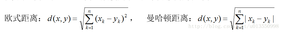
在KNN中,通过计算待测样本和训练样本的特征值之间的差异(距离)作为对象之间的相似性指标,一般使用欧氏距离或曼哈顿距离:
k-近邻算法优点是精度高、对异常值不敏感、无数据输入假定。缺点是计算复杂度高、空间复杂度高。适用数据范围为数值型和标称型。
算法描述
1)计算测试数据与各个训练数据之间的距离;
2)按照距离的递增关系进行排序;
3)选取距离最小的K个点;
4)确定前K个点所在类别的出现频率;
5)返回前K个点中出现频率最高的类别作为测试数据的预测分类。
# -*- coding: utf-8 -*-
""" k-Nearest Neighbors
Created on Mon Jan 23 12:56:00 2017

@author: xieyuxi
"""
from numpy import *
import operator
import numpy as np

def createDataSet():
    group = array([[1.0, 1.1],[1.0,1.0],[0,0],[0,0.1]])
    lables = ['A','A','B','B']
    return group, lables
    print group, lables


createDataSet()

""" Classify the unknown vector input into defined classes
1、calculate the distance between inX and the current point
2、sort the distances in increasing order
3、take k items with lowest distances to inX
4、find the majority class among these items
5、return the majority class as our prediction for the class of inX

Args:
     inX : the input vector to classify
     dataSet : the full matrix of training examples
     labels : a vector of labels from the training examples
     k : the number of nearest neighbors to use in the voting

Attention:
    The labels vector should have as many elements in it
    as there are rows in the dataSet matrix.

Returns:
     the majority class as our prediction for the class of inX

Raises:
    None
"""
def classify0(inX, dataSet, labels, k):
    # shape是numpy的数组的一个属性,表示数组的维度
    # 比如一个 n x m的数组 Y(n 行 m列),Y.shape表示(n,m)
    # 所以 Y.shape[0]等于 n, Y.shape[1]等于 m
    # dataSet是4X2的数组,所以此处dataSetSize等于4
    dataSetSize = dataSet.shape[0]      # 4
    # 1、先将一维矩阵扩展和测试矩阵的维度一样
    # 2、将新生成的待测矩阵同测试矩阵进行矩阵减法,再将矩阵的差的平方和开根得到距离
    # 3、将距离排序并返回
#==============================================================================
#     1、 tile(A, reps):reps的数字从后往前分别对应A的第N个维度的重复次数。
#        如(A,2)表示A的列变量重复2遍,
#           tile(A,(2,3))表示A的行变量重复2遍,列变量重复3遍
#           tile(A,(2,2,3))表示A的第一个维度重复2遍,第二个维度重复2遍,
#           第三个维度重复3遍。
#           Examples:
#     ----------------------------------------
#     # a = np.array([0, 1, 2])
#     # np.tile(a, 2)
#     array([0, 1, 2, 0, 1, 2])
#     # np.tile(a, (2, 3))
#     array([[0, 1, 2, 0, 1, 2, 0, 1, 2],
#            [0, 1, 2, 0, 1, 2, 0, 1, 2]])
#     ----------------------------------------
#     # b = np.array([[1, 2], [3, 4]])
#     # np.tile(b, 2)
#     array([[1, 2, 1, 2],
#            [3, 4, 3, 4]])
#     # np.tile(b, (2, 1))
#     array([[1, 2],
#            [3, 4],
#            [1, 2],
#            [3, 4]])
#
#     2、diffMat矩阵:先将输入的值复制到和训练样本同行,再做减法
# 以[0,0]为例:
# [0,0] to array([[0, 0]       [[0, 0]   [[1.0,1.1]           [[-1.  -1.1]
#                 [0, 0]  to   [0, 0] -  [1.0,1.0]    to       [-1.  -1. ]
#                 [0, 0]       [0, 0]    [0,0]                 [ 0.   0. ]
#                 [0, 0]])     [0, 0]]   [0,0.1]]              [ 0.  -0.1]]
#==============================================================================

    diffMat = tile(inX, (dataSetSize,1)) - dataSet
    # 其中矩阵的每一个元素都做平方操作
    #    [[ 1.    1.21]
    #     [ 1.    1.  ]
    #     [ 0.    0.  ]
    #     [ 0.    0.01]]
    sqDiffMat = diffMat**2
    # axis=0, 表示列。 axis=1, 表示行。
    # example:
    # c = np.array([[0, 2, 1], [3, 5, 6], [0, 1, 1]])
    # c.sum() = 19
    # c.sum(axis=0) =[3 8 8],即将矩阵的行向量想加后得到一个新的一维向量
    # c.sum(axis=1) =[3,14,2], 即每个向量将自己内部元素加和作新一维向量里的一个元素
    # 此处已经将每一个行向量中的每一个元素都做了平方操作,并求和得到每一个向量之和
    # 得到一个一维数组,其中有四个元素分别对应了输入元素与 4个测试样本的平方距离
    sqDistances = sqDiffMat.sum(axis=1)     # [ 2.21  2.    0.    0.01]
    # 将平方距离开方
    distances = sqDistances**0.5 # [ 1.48660687  1.41421356  0.          0.1 ]
    # argsort函数返回的是数组值从小到大的索引值
    # examples:
    #     # x = np.array([3, 1, 2])
    #     # np.argsort(x)
    #         array([1, 2, 0]) 数值1对应下表1,数值2对应下表2,数值3,对应下标0
    # [1.48660687  1.41421356  0.0  0.1 ] to [2 3 1 0]
    sortedDistIndex = distances.argsort()   # [2 3 1 0]
    # 建造一个名为classCount的字典,Key是label,value是这个label出现的次数
    classCount={}
    for i in range(k):
        # 这里很巧妙的地方在于,一开始测试数组和Label的位置是一一对应的
        # 所以这里可以通过上面获得的测试数组的下标index获得对应的分类labels[index]
        voteLabel = labels[sortedDistIndex[i]]
        # 这里将每一个[label : Value]赋值,Value为计算VoteLabel出现的次数
        # 如果Label不在字典classCount中时,get()返回 0,存在则value加 1
        classCount[voteLabel] = classCount.get(voteLabel,0) + 1

    # 根据字典classCount中的Value值对字典进行排序,选出出现次数最多的Label
    #       sorted(iterable, cmp=None, key=None, reverse=False)
    #       return new sorted list
    #       1、iterable:是可迭代类型的对象(这里的字典通过iteritems()进行迭代)
    #       2、cmp:用于比较的函数,比较什么由key决定,一般用Lamda函数
    #       3、key:用列表元素的某个属性或函数进行作为关键字,迭代集合中的一项;
    #               operator.itemgetter(1)表示获得对象的第一个域的值(这里指value)
    #       4、reverse:排序规则。reverse = True 降序 或者 reverse = False 升序。
    #
    #       return: 一个经过排序的可迭代类型对象,与iterable一样。
    #               这里返回排好序的[Label:value], 即 [('B', 2), ('A', 1)]
    sortedClassCount = sorted(classCount.iteritems(),
                              key=operator.itemgetter(1), reverse=True)
    # 返回可迭代对象的第一个域的第一值,也就是出现次数最多的Label
    # sortedClassCount[0][1] 表示第一个域的第二个值,就是出现最多次数Label出现次数
    return sortedClassCount[0][0]
本案例的数据被置于txt文件中,所以需要我们将数据从txt文件中抽出并做处理。所以我们准备函数file2matrix()将txt的数据转换为矩阵方便我们后面做运算。
""" Parsing data from a text file
Change the text file data to the format so that the classifier can accept and use it

Args:
     filename string

Returns:
    A matrix of training examples,
    A vector of class labels

Raises:
    None
"""
def file2matrix(filename):
    # 根据文件名打开文件
    fr = open(filename)
    # 读取每一行的数据
    # txt文件中的数据类似:"40920      8.326976    0.953952    largeDoses"W
    arrayOlines = fr.readlines()
    # 得到文件行数
    numberOfLines = len(arrayOlines)
    # 创建返回的Numpy矩阵
    # zeros(a) 仅有一个参数时,创建一个一维矩阵,一行 a 列
    # zeros(a, b) 创建一个 a X b 矩阵, a 行 b 列
    # 这里取了数据的行数和前三个特征值(前三个是特征,第四个个是类别)创建一个矩阵
    returnMat = zeros((numberOfLines,3))
    # 建造一个名为 classLabelVector 的 List 用来存放最后列的Label
    classLabelVector = []
    # 这里的 index 指的是矩阵的第几行,从 0 开始
    index = 0
    #( 以下三行) 解析文件数据到列表
    for line in arrayOlines:
        # 去掉文本中句子中的换行符"/n",但依然保持一行四个元素
        line = line.strip()
        # 以 ‘\t’(tab符号)分个字符串,文本中的数据是以tab分开的
        # 另外需要注意 split() 函数返回一个 List对象
        #       如:['30254', '11.592723', '0.286188', '3']
        listFromLine = line.split('\t')
        # 选取前listFromLine的三个元素,存储在特征矩阵中
        # returnMat[index,:]这里需要注意,因为returnMat是一个矩阵
        #       其中的 index指的是矩阵中的第几个list
        #       例如 listMat = [[list1]
        #                       [list2]
        #                       [list3]
        #                       ......
        #                       [listn]]
        #       listMat[0]表示的是矩阵listMat中的第1行,即 [list1]
        #       listMat[2,:] 表示的是矩阵listMat中的第3行的所有元素
        #       listMat[2,0:2] 表示矩阵listMat中的第3行下标为 0和1两个元素
        #
        # listFromLine[0:3]切片开始于0、停止于3,也就是取了下标为0,1,2的元素
        # 将listFromLine[0:3]的第0号到2号元素赋值给特征矩阵returnMat对应特征中
        returnMat[index,:] = listFromLine[0:3]
        # listFromLine[-1] 取listFromLine的最后一列标签类(将其强行转换为int类型)
        # 同时将该类别标签按顺序加入到标签向量classLabelVector中
        classLabelVector.append(int(listFromLine[-1]))
        # index加 1,矩阵存取下一个list
        index += 1

    return returnMat,classLabelVector
在这先根据特征值,利用Matplotlib绘制类别的散点图。
import matplotlib
# matplotlib的pyplot子库提供了和matlab类似的绘图API,方便用户快速绘制2D图表。
import matplotlib.pyplot as plt
# 我们先利用写好的KNN.py文件中的file2matrix()函数将数据转为矩阵
datingDataMat, datingLabels = KNN.file2matrix(filename)
# 这里创建了一个新的 figure,我们要在上面作图
fig = plt.figure()
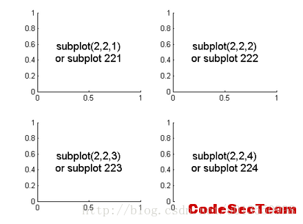
# add_subplot(111)相当于在figure上添加子图
# 其中 111 的意思是,将子图切割成 1行 1列的图,并在第 1 块上作画
# 所以这里只有一副画
# 再举个例子 add_subplot(22x),将子图切割成 2行 2列的图,并在第 X 块上作画
ax = fig.add_subplot(111)
# 利用scatter()函数分别取已经处理好的矩阵datingDataMat的第一列和第二列数据
# 并用不同颜色将类别标识出来
ax.scatter(datingDataMat[:,0], datingDataMat[:,1],
15.0*array(datingLabels), 15.0*array(datingLabels))
# 展示我们做好的 figure
plt.show()下图是很好地解释add_subplot(22x):
根据矩阵第一列和第二列数据可以获得以下带有颜色类别区分的散点图:
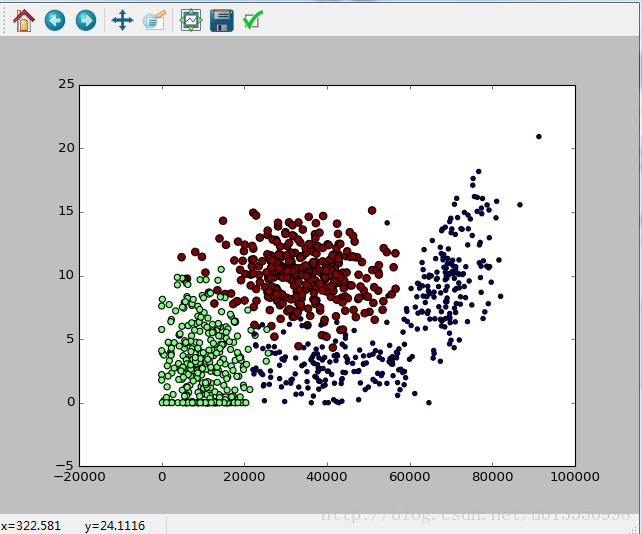
(红色的点表示非常喜欢,绿色的点表示一般喜欢,蓝色的点表示并不喜欢)
观察上图我们不难发现一个问题,如果当某一个特征值与其他的特征值的差异过大的话,如果不加权重或各特征权重均衡的话,很可能会影响到最后的分类,比如例子中的飞行距离,远远大于其他两个特征值,在这种情况下,特征的距离就会受飞行距离特征值得影响。所以我们需要将数据进行归一化,即将所有数据都变为 0~1 之间的数,目的是让数据的影响都能比较均衡。
""" Normalizing numeric values
Normalize the data to values between 0 and 1.

Formula:
    newValue = (oldValue-min)/(max-min)
In the normalization procedure, the variables min and max are the
smallest and largest values in the dataset.

Args:
     dataSet: the data set to be normalized

Returns:
    A normalized data set

Raises:
    None
"""
def autoNorm(dataSet):
    # min(0)取矩阵每一列的最小值
    # min(1)取矩阵每一行的最小值
    # Examples:
    #     array([[1,2]
    #            [3,4]
    #            [5,6]])
    #       min(array,0) = [1,2]
    #       min(array,1) = [1,3,5]
    # 这里同: minVals = np.min(dataSet,0)
    # 返回的是一个一维矩阵
    minVals = dataSet.min(0)
    # max(0)取矩阵每一列的最大值
    # max(1)取矩阵每一列的最大值
    # 返回的是一个一维矩阵
    maxVals = dataSet.max(0)
    # ranges也是一个一维矩阵
    ranges = maxVals - minVals
    # shape(dataSet) 返回一个记录有矩阵维度的tuple
    # 例如:np.shape([[1, 2]]) = (1, 2)
    # zeros(shape)返回一个具有 shape 维度的矩阵,并且所有元素用 0 填充
    normDataSet = zeros(shape(dataSet))
    # m 表示 dataSet 矩阵的行数
    # dataSet.shape[1] 表示矩阵的列数
    m = dataSet.shape[0]
    # tile(minVals, (m,1)) 首先将 minVals 复制为 m 行的矩阵
    # examples:
    #    if   minVals = [[1,2,3]]
    #         tile(minVals, (3,1))(行数复制 3 遍,列保持不变)
    #    return [[1,2,3]
    #            [1,2,3]
    #            [1,2,3]]
    normDataSet = dataSet - tile(minVals, (m,1))
    # 同上,将 一维矩阵 ranges 复制 m行,再让矩阵中的元素做商
    normDataSet = normDataSet/tile(ranges, (m,1))
    # 返回归一化的矩阵,最大与最小值的差值矩阵,和最小值矩阵
    return normDataSet, ranges, minVals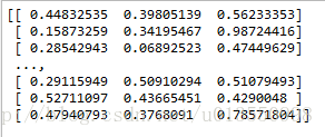
(上图为归一化后的特征值)
我自己的博客地址为:谢雨熹的学习博客
欢迎大家来交流!
Talk is cheap, show me your code!