一、说明

多项式回归可以识别自变量和因变量之间的非线性关系。本文是关于回归、梯度下降和 MSE 系列文章的第三篇。前面的文章介绍了简单线性回归、回归的正态方程和多元线性回归。

二、多项式回归

多项式回归用于最适合曲线拟合的复杂数据。它可以被视为多元线性回归的子集。

请注意，X₀ 是偏差的一列;这允许在第一篇文章中讨论的广义公式。使用上述等式，每个“自变量”都可以被视为 X₁ 的指数版本。

这允许从多元线性回归使用相同的模型，因为只需要识别每个变量的系数。可以创建一个简单的三阶多项式模型作为示例。其等式如下：

模型、梯度下降和 MSE 的广义函数可用于前面的文章：

# line of best fit
def model(w, X):
  """
    Inputs:
      w: array of weights | (num features, 1)
      X: array of inputs  | (n samples, num features)

    Output:
      returns the output of X@w | (n samples, 1)
  """

  return torch.matmul(X, w)

# mean squared error (MSE)
def MSE(Yhat, Y):
  """
    Inputs:
      Yhat: array of predictions | (n samples, 1)
      Y: array of expected outputs | (n samples, 1)
    Output:
      returns the loss of the model, which is a scalar
  """
  return torch.mean((Yhat-Y)**2) # mean((error)^2)

# optimizer
def gradient_descent(w):
  """
    Inputs:
      w: array of weights | (num features, 1)

    Global Variables / Constants:
      X: array of inputs  | (n samples, num features)
      Y: array of expected outputs | (n samples, 1)
      lr: learning rate to scale the gradient

    Output:
      returns the updated weights
  """ 

  n = X.shape[0]

  return w - (lr * 2/n) * (torch.matmul(-Y.T, X) + torch.matmul(torch.matmul(w.T, X.T), X)).reshape(w.shape)

三、创建数据

现在，所需要的只是一些用于训练模型的数据。可以使用“蓝图”功能，并且可以添加随机性。这遵循与前面文章相同的方法。蓝图如下所示：

可以创建大小为（800， 4）的训练集和大小为（200， 4）的测试集。请注意，除偏差外，每个特征都是第一个特征的指数版本。

import torch

torch.manual_seed(5)
torch.set_printoptions(precision=2)

# features
X0 = torch.ones((1000,1))
X1 = (100*(torch.rand(1000) - 0.5)).reshape(-1,1) # generates 1000 random numbers from -50 to 50
X2, X3 = X1**2, X1**3
X = torch.hstack((X0,X1,X2,X3))

# normal distribution with a mean of 0 and std of 8
normal = torch.distributions.Normal(loc=0, scale=8)

# targets
Y = (3*X[:,3] + 2*X[:,2] + 1*X[:,1] + 5 + normal.sample(torch.ones(1000).shape)).reshape(-1,1)

# train, test
Xtrain, Xtest = X[:800], X[800:]
Ytrain, Ytest = Y[:800], Y[800:]

定义初始权重后，可以使用最佳拟合线绘制数据。

torch.manual_seed(5)
w = torch.rand(size=(4, 1))
w

tensor([[0.83],
        [0.13],
        [0.91],
        [0.82]])

import matplotlib.pyplot as plt

def plot_lbf():
  """
    Output:
      prints the line of best fit in comparison to the train and test data
  """

  # plot the train and test sets
  plt.scatter(Xtrain[:,1],Ytrain,label="train")
  plt.scatter(Xtest[:,1],Ytest,label="test")

  # plot the line of best fit
  X1_plot = torch.arange(-50, 50.1,.1).reshape(-1,1) 
  X2_plot, X3_plot = X1_plot**2, X1_plot**3
  X0_plot = torch.ones(X1_plot.shape)
  X_plot = torch.hstack((X0_plot,X1_plot,X2_plot,X3_plot))

  plt.plot(X1_plot.flatten(), model(w, X_plot).flatten(), color="red", zorder=4)

  plt.xlim(-50, 50)
  plt.xlabel("$X$")
  plt.ylabel("$Y$")
  plt.legend()
  plt.show()

plot_lbf()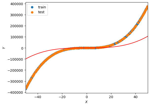

四、训练模型

为了部分最小化成本函数，可以使用 5e-11 和 500，000 epoch 的学习率与梯度下降一起使用。

lr = 5e-11
epochs = 500000

# update the weights 1000 times
for i in range(0, epochs):
  # update the weights
  w = gradient_descent(w)

  # print the new values every 10 iterations
  if (i+1) % 100000 == 0:
    print("epoch:", i+1)
    print("weights:", w)
    print("Train MSE:", MSE(model(w,Xtrain), Ytrain))
    print("Test MSE:", MSE(model(w,Xtest), Ytest))
    print("="*10)

plot_lbf()

epoch: 100000
weights: tensor([[0.83],
        [0.13],
        [2.00],
        [3.00]])
Train MSE: tensor(163.87)
Test MSE: tensor(162.55)
==========
epoch: 200000
weights: tensor([[0.83],
        [0.13],
        [2.00],
        [3.00]])
Train MSE: tensor(163.52)
Test MSE: tensor(162.22)
==========
epoch: 300000
weights: tensor([[0.83],
        [0.13],
        [2.00],
        [3.00]])
Train MSE: tensor(163.19)
Test MSE: tensor(161.89)
==========
epoch: 400000
weights: tensor([[0.83],
        [0.13],
        [2.00],
        [3.00]])
Train MSE: tensor(162.85)
Test MSE: tensor(161.57)
==========
epoch: 500000
weights: tensor([[0.83],
        [0.13],
        [2.00],
        [3.00]])
Train MSE: tensor(162.51)
Test MSE: tensor(161.24)
==========

即使有 500，000 个 epoch 和极小的学习率，该模型也无法识别前两个权重。虽然当前的解决方案非常准确，MSE为161.24，但可能需要数百万个epoch才能完全最小化它。这是多项式回归梯度下降的局限性之一。

五、正态方程

作为替代方案，可以使用第二篇文章中的正态方程直接计算优化权重：

def NormalEquation(X, Y):
  """
    Inputs:
      X: array of input values | (n samples, num features)
      Y: array of expected outputs | (n samples, 1)
      
    Output:
      returns the optimized weights | (num features, 1)
  """
  
  return torch.inverse(X.T @ X) @ X.T @ Y

w = NormalEquation(Xtrain, Ytrain)
w

tensor([[4.57],
        [0.98],
        [2.00],
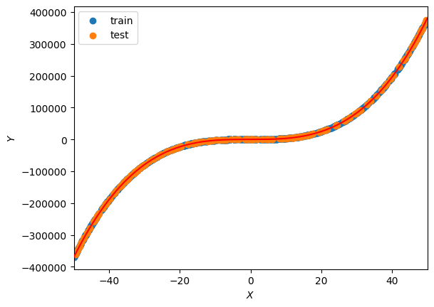
        [3.00]])

正态方程能够立即识别每个权重的正确值，并且每组的MSE比梯度下降时低约100点：

MSE(model(w,Xtrain), Ytrain), MSE(model(w,Xtest), Ytest)

(tensor(60.64), tensor(63.84))

六、结论

通过实现简单线性、多重线性和多项式回归，接下来的两篇文章将介绍套索和岭回归。这些类型的回归在机器学习中引入了两个重要概念：过拟合和正则化。

参考文章：

亨特·菲利普斯

Python 中的机器学习简介：多项式回归