[Machine Learning]多元线性回归与多项式回归Python实现

在一元线性回归中，输入特征只有一维，
$h_{θ}=θ_0 + x_1θ_1$ , 对于多元特征，假设函数推广到了
$h_{θ}=θ_0 + x_1θ_1+ x_2θ_2+ x_3θ_3+...+ x_mθ_m$
对于非线性的一维数据，用线性回归拟合结果并不好，可以采用多项式回归，手动增加特征，例如如下4种多项式拟合
$h_{θ}=θ_0 + θ_1x_1+θ_2x_1^2$ (1)
$h_{θ}=θ_0 + θ_1x_1+θ_2x_1^2θ_2+θ_3x_1^3$ (2)
$h_{θ}=θ_0 + θ_1x_1+θ_2log(x_1)$ (3)
$h_{θ}=θ_0 + θ_1x_1+θ_2\sqrt x_1$ (4)
我们可以将多项式回归转换为多元回归，例如在式(1)中，可以令 $x_1^2$ 为 $x_2$ ，此时假设函数为
$h_{θ}=θ_0 + θ_1x_1+θ_2x_2$ ，
根据梯度下降求出 $θ_0，θ_1，θ_2$ 。
在上一篇博文一元线性回归中，
(http://blog.csdn.net/murphy_coolcoder/article/details/78946003)
最终拟合出的曲线如图所示

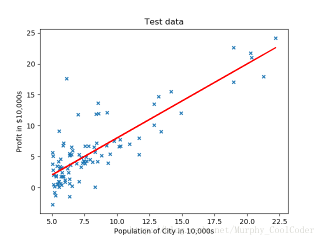
如果我们想采用如下曲线拟合
$h_{θ}=θ_0 + θ_1x_1+θ_2log(x_1)$

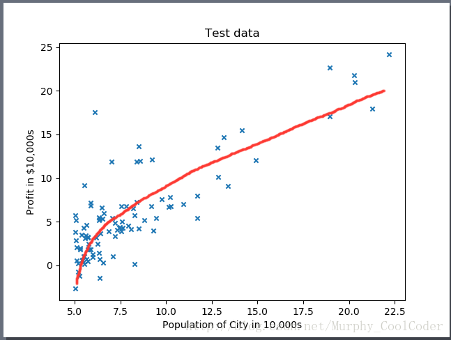
或者如下二次函数拟合
$h_{θ}=θ_0 + θ_1x_1+θ_2x_1^2$

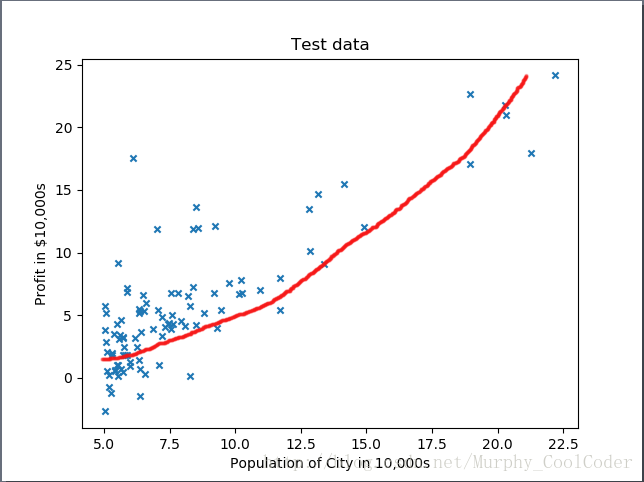
则需要对输入数据增加一个对应的特征 $X_2$ , 若采用 log则
$X_2 = log(X_1)$ ,若采用二次函数则 $X_2 = X_1^2$ ,然后进行梯度下降，得到 $θ_0，θ_1，θ_2$ 。
这里有几个trick要注意，
1).增加了一个特征之后，我们实际上将数据上升到3维空间，在做梯度下降之前，我们对训练样本先要进行归一化，尤其如果是高次多项式，特征之间数值差别很大，不做归一化梯度下降会很慢，而且还容易停止在局部最优而不是全局最优，不利于后续数值处理。
2).由于多项式回归是单一特征的多项式和，因此可以在二维空间展示出来，就如上图二所示。要在二维空间展示多项式曲线，对于输入数据要先做归一化，再增加特征向量。但此时会有一个问题存在，如果是多项式是log函数，在使用z-score归一化的情况下，没法在二维空间展示。因为采用z-score归一化的一维特征 $Norm_X_1$ 会有负值存在，此时在此基础之上增加 $log(Norm_X_1)$ 特征会无效. 只能在三维空间展示。当然如果可以采用某种归一化方法，使其一维特征经过归一化后没有负值和0值存在，那么二维特征 $log(Norm_X_1)$ 便可以运算，则也可以在二维空间展示出来，本文不做深入探讨。
3). 对于测试样本，测试样本的归一化参数要使用训练样本的归一化参数。如训练样本采用z-score归一化方法，均值u1, 方差sigma1。对于测试样本，测试样本的归一化参数不应使用自身的均值u2和方差sigma2而应使用训练样本的均值u1 和方差sigma1 作为归一化参数。
4). 在使用Matplotlib 绘制拟合函数时，建议使用散点图绘制，可以避免参数顺序变化带来的图像错乱。

源代码如下，数据集
训练样本数据https://pan.baidu.com/s/1nuM66mt
note：本代码对数据集采用8：2的比例作为训练样本与测试样本，由于使用了np.random.shuffle()函数，每次运行的结果不尽相同，如要想要修改训练样本与测试样本的比例或者固定样本选择顺序，可以修改类中 sampleDivde 方法，参数“ratio”可以调整比例，注释掉np.random.shuffle()函数可以固定训练样本选择顺序。

import numpy as np
import matplotlib.pyplot as plt
from mpl_toolkits.mplot3d import Axes3D
from scipy.interpolate import spline

class LinearRegression:
    def sampleDivde(self,data_X,data_Y,feature_num,ratio):
        combineMatix = np.append(data_X.T,data_Y).reshape(feature_num+1,data_X.shape[0]).T
        np.random.shuffle(combineMatix)
        m = int(data_X.shape[0]*ratio)
        train_X = combineMatix[:m,:feature_num]
        train_Y = combineMatix[:m,feature_num]
        test_X =combineMatix[m:,:feature_num]
        test_Y = combineMatix[m:,feature_num]
        return train_X,train_Y,test_X,test_Y
    def featureScale(self, data_X):
        u = np.mean(data_X,0)
        sigma = np.std(data_X,0)
        newData = (data_X - u)/sigma
        return newData, u, sigma
    def testScale(self,data_X,u,sigma):
        newData = (data_X - u) / sigma
        return newData

    def biasAdd(self, data_X, feature_num):
        biasX = np.ones(data_X.shape[0])
        newX = np.append(biasX, data_X.T).reshape(feature_num + 1, data_X.shape[0]).T
        return newX
    def featureAdd(self, data_X, model, feature_num):
        if model == 0:
            return data_X
        if model == 1:
            feature_add = np.log2(data_X)
        elif model == 2:
            feature_add = np.sqrt(data_X)
        elif model == 3:
            feature_add = np.power(data_X,2)
        X = np.append(data_X, feature_add).reshape(feature_num + 1, data_X.shape[0]).T
        return X
    def costFunc(self,theta,data_X,data_Y):
        m = data_X.shape[0]
        J = np.dot((np.dot(theta,data_X.T).T- data_Y).T,np.dot(theta,data_X.T).T-data_Y)/(2*m)
        return J
    def gradientDescent(self,theta,data_X,data_Y,alpha,num_iters):
        m = data_X.shape[0]
        for i in range(num_iters):
            theta = theta - np.dot(data_X.T,np.dot(theta.T,data_X.T).T- data_Y)*alpha/m
        return theta
    def error(self,theta,test_X,Y_label):
        test_Y = np.dot(theta,test_X.T)
        error = sum(test_Y-Y_label)/Y_label.shape
        return error
    def learningRateCheck(self,theta,data_X,data_Y,alpha):
        m = data_Y.shape[0]
        j_X = []
        j_Y = []
        for i in range(0,100,5):
            j_X.append(i)
            for j in range(i):
                theta = theta - np.dot(data_X.T, np.dot(theta.T, data_X.T).T - data_Y) * alpha / m
            j_Y.append(self.costFunc(theta,data_X,data_Y))
        xNew = np.linspace(min(j_X), max(j_X), 300)
        ySmooth = spline(j_X,j_Y,xNew)
        plt.plot(xNew,ySmooth, color = 'red')
        plt.show()
if __name__ =='__main__':
    path = 'Housedata.txt'
    fr = open(path, 'r+')
    x = []
    y = []
    for line in fr:
        items = line.strip().split(',')
        x.append(float(items[0]))
        y.append(float(items[1]))
    test = LinearRegression()
    data_X = np.array(x)
    data_Y = np.array(y)
    a = data_X
    z = data_Y
    train_X, train_Y, test_X, test_Y = test.sampleDivde(data_X, data_Y,1,0.8) #no bias
    #Linear regression data pre-processing
    norm_train_X,u,sigma = test.featureScale(train_X)
    biasnorm_train_X = test.biasAdd(norm_train_X,1)
    norm_test_X = test.testScale(test_X,u,sigma)
    biastest_X = test.biasAdd(norm_test_X,1)
    # gradient Descent
    theta = np.zeros(biasnorm_train_X.shape[1])
    theta_Results = test.gradientDescent(theta, biasnorm_train_X, train_Y, 0.1, 1500)
    #Plot data
    X = train_X
    Y = np.dot(theta_Results,  biasnorm_train_X.T)
    plt.subplot(211)
    plt.plot(X, Y, color='red')
    plt.scatter(data_X, data_Y, s=20, marker="x") #plot raw data
    plt.title('Linear fit')

    #Polyomial Regression#
    #************1. Quadratic fit*********
    # train data used for train
    Q_feature_add_train_X = test.featureAdd(train_X, 3, 1)  # 3 in featureAdd function represent squre
    Q_norm_train_X, Q_u, Q_sigma = test.featureScale(Q_feature_add_train_X)
    Q_biasnorm_train_X = test.biasAdd(Q_norm_train_X, 2)
    # test data used for train
    Q_feature_add_test = test.featureAdd(test_X, 3, 1)
    Q_norm_test = test.testScale(Q_feature_add_test, Q_u, Q_sigma)
    Q_bias_test_X = test.biasAdd(Q_norm_test, 2)
    #gradient Descent
    theta = np.zeros(Q_biasnorm_train_X.shape[1])
    Q_theta_Results = test.gradientDescent(theta, Q_biasnorm_train_X, train_Y, 0.1, 1500)
    #data used for plot,which is featureScale first, than add feature X2.
    Q_norm_X,p_u,p_sigma = test.featureScale(train_X)
    Q_feature_add_norm_X = test.featureAdd(Q_norm_X, 3, 1)
    Q_biasnorm_X = test.biasAdd(Q_feature_add_norm_X, 2)
    # Plot data
    X = train_X
    Y = np.dot(Q_theta_Results, Q_biasnorm_X.T)
    plt.subplot(212)
    plt.scatter(X, Y, color='red')
    plt.scatter(data_X, data_Y, s=20, marker="x")  # plot raw data
    plt.title('Quadratic fit')
    plt.show()

    # ************3. Log fit*********
    # train data used for train
    L_feature_add_train_X = test.featureAdd(train_X, 1, 1)  # 1 in featureAdd function represent  log
    L_norm_Train_X,L_u,L_sigma = test.featureScale(L_feature_add_train_X)
    L_biasTrain_X = test.biasAdd(L_norm_Train_X, 2)
    # test data used for train
    L_feature_add_test_X = test.featureAdd(test_X, 1, 1)
    L_norm_Test_X = test.testScale(L_feature_add_test_X,L_u,L_sigma)
    L_biasTest_X = test.biasAdd(L_norm_Test_X, 2)
    # gradient Descent
    theta = np.zeros(L_biasTrain_X.shape[1])
    L_theta_Results = test.gradientDescent(theta, L_biasTrain_X, train_Y, 0.2, 1500)
    # Plot 3D data
    ax = plt.subplot(111, projection='3d')
    X = train_X
    Y = np.log2(train_X)
    Z = np.dot(L_theta_Results, L_biasTrain_X.T)
    ax.scatter(X,Y,Z, color='g')
    ax.scatter(X,Y,train_Y, c='r')  # 绘制数据点
    ax.set_zlabel('Z')  # 坐标轴
    ax.set_ylabel('Y')
    ax.set_xlabel('X')
    plt.show()

    ######Error  check########
    error = test.error(theta_Results, biastest_X, test_Y)
    print("Linear regression error is:",error)
    Q_error = test.error(Q_theta_Results, Q_bias_test_X, test_Y)
    print("Quadratic Polyomial Regression error is:",Q_error)
    L_error = test.error(L_theta_Results, L_biasTest_X, test_Y)
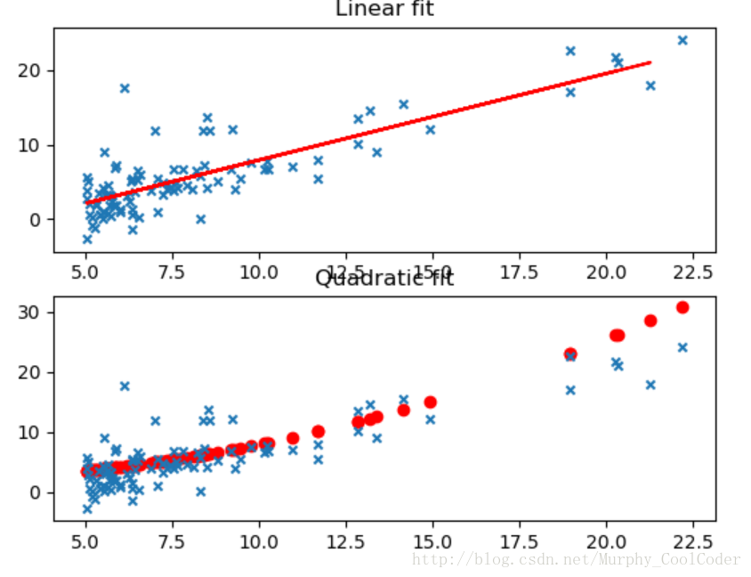
    print("Log Polyomial Regression error is:",L_error)

二次拟合结果与一元线性回归拟合比较

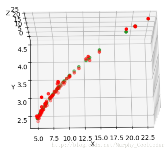
Log 拟合三维图像

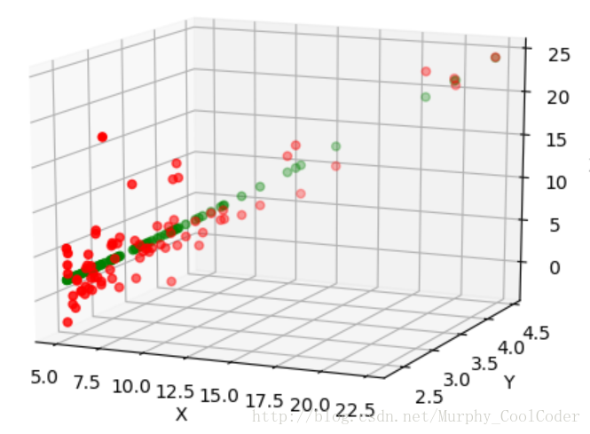
拖动三维图像，可以看出X与Y 的对数关系
这里写图片描述

由于采取了随机策略，由于训练样本选择的不同，三种方法的误差比较也不尽相同。某些情况下Log拟合最优，某些情况下线性回归反而表现要好。这是与数据集分不开的。就本实例的数据集来说，三种拟合方式差别不大。对应于不同的数据集，采用不同的方式，甚至更高次的多项式拟合，要根据具体问题来分析。本文只是给简要分析了一下多项式拟合和多元线性回归二者之间的关系以及我在调试代码过程中所遇到的问题，以供参考。

[Machine Learning]多元线性回归与多项式回归Python实现

猜你喜欢