Python实现多项式回归实战——以及与线性回归的拟合效果对比

对于给出的数据做出散点图，可以大致看出模型是否适合做线性回归，但是，线性回归一定是拟合最好的模型吗？答案是否定的。有时候，多项式回归会得出拟合效果更好的模型，但是也需要注意过拟合的线性。

下面，还是以房屋面积预测房屋价格的数据为例：

读取数据，绘制散点图：

 多项式回归
import matplotlib.font_manager as fm
import matplotlib.pyplot as plt
from sklearn import linear_model
import numpy as np
from sklearn.linear_model import LinearRegression #导入线性回归模型
from sklearn.preprocessing import PolynomialFeatures # 导入多项式回归模型

# 字体
myfont = fm.FontProperties(fname='C:\Windows\Fonts\simsun.ttc')
# plt.figure()  # 实例化作图变量
plt.title('房价面积价格样本', fontproperties = myfont)  # 图像标题
plt.xlabel('面积(平方米)', fontproperties = myfont)  # x轴文本
plt.ylabel('价格(万元)', fontproperties = myfont)  # y轴文本
# plt.axis([30, 400, 100, 400])
plt.grid(True)  # 是否绘制网格线

# 训练数据（给定的房屋面积x和价格y）
X = [[50], [100], [150], [200], [250], [300]]
y = [[150], [200], [250], [280], [310], [330]]

# 做最终效果预测的样本
X_test = [[250], [300]]  # 用来做最终效果测试
y_test = [[310], [330]]  # 用来做最终效果测试

# 绘制散点图
# plt.plot(X, y, 'b.')#点
# plt.plot(X, y, 'b-')#线
plt.scatter(X, y, marker='*',color='blue',label='房价面积价格样本')
# plt.show()

先做出线性模型：

# 线性回归
model = LinearRegression()
model.fit(X,y)
# 模型拟合效果得分
print('一元线性回归 r-squared',model.score(X_test,y_test))
x2=[[30],[400]] # 所绘制直线的横坐标x的起点和终点
y2=model.predict(x2)
plt.plot(x2,y2,'g-')  # 绿色的直线
# plt.show()

做出二项式回归模型，看拟合效果，同线性模型进行比较：

# 二次多项式回归
# 实例化一个二次多项式特征实例
quadratic_featurizer=PolynomialFeatures(degree=2)
# 用二次多项式对样本X值做变换
X_train_quadratic = quadratic_featurizer.fit_transform(X)
# 创建一个线性回归实例
regressor_model=linear_model.LinearRegression()
# 以多项式变换后的x值为输入，带入线性回归模型做训练
regressor_model.fit(X_train_quadratic,y)
# 设计x轴一系列点作为画图的x点集
xx=np.linspace(30,400,100)
# 把训练好X值的多项式特征实例应用到一系列点上,形成矩阵
xx_quadratic = quadratic_featurizer.transform(xx.reshape(xx.shape[0], 1))

yy_predict = regressor_model.predict(xx_quadratic)

# 用训练好的模型作图
plt.plot(xx, yy_predict, 'r-')


X_test_quadratic = quadratic_featurizer.transform(X_test)
print('二次回归     r-squared', regressor_model.score(X_test_quadratic, y_test))
# plt.show()  # 展示图像

得到图像：

红色的线就是二项式的回归模型，可以看出它是比线性回归模型对本案例的数据拟合效果要好一些，二者的拟合效果得分分别为：

那么，当前的二次回归是否是最好的呢？我们再做三次回归看一下：

# 三次回归
cubic_featurizer = PolynomialFeatures(degree=3)
X_train_cubic = cubic_featurizer.fit_transform(X)
regressor_cubic = LinearRegression()
regressor_cubic.fit(X_train_cubic, y)
xx_cubic = cubic_featurizer.transform(xx.reshape(xx.shape[0], 1))
plt.plot(xx, regressor_cubic.predict(xx_cubic))

X_test_cubic = cubic_featurizer.transform(X_test)
print('三次回归     r-squared', regressor_cubic.score(X_test_cubic, y_test))
plt.show()  # 展示图像

得到的图形为：

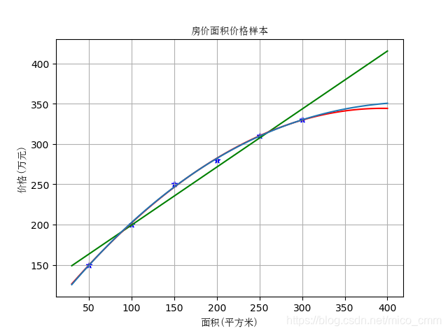
从图形来看，它和二次回归模型的拟合效果不相上下，分辨不出孰好孰坏，下面看一下拟合得分。

图形模型拟合效果得分为：

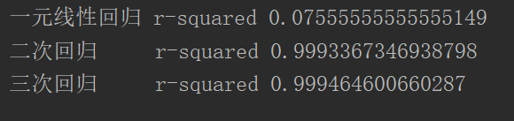
可以看出，三次回归的模型拟合得分比二次回归高，但是相差不多，从图形看来二者拟合效果都很好，因此我们在此种情况下选择二次回归，原因为三次回归可能出现了过拟合的现象。

Python实现多项式回归实战——以及与线性回归的拟合效果对比

读取数据，绘制散点图：

先做出线性模型：

做出二项式回归模型，看拟合效果，同线性模型进行比较：

那么，当前的二次回归是否是最好的呢？我们再做三次回归看一下：

猜你喜欢