Towards Real-Time Multi-Object Tracking

Towards Real-Time Multi-Object Tracking

Abstract

The components of traditional MOT strategies which follows the tracking-by-detection paradigm¹:

• detection model
• appearance embedding model
• data association

The shortcomings of traditional MOT strategies:

• poor efficiency

While in this paper, the author proposed a new method to solve the problem which allows detection and appearance embedding to be learned in a shared model (single-shot detector). Further more, the author propose a simple and fast association method.

code

1 Introduction

MOT—— Predicting trajectories of multiple targets in video sequences.

tracking-by-detection—— SDE² :

• Detection—— Localize targets. (detector)
• Association. (re-ID model)
• Problem—— Inefficient.

Solution: Integrate the two tasks into a single network (Faster R-CNN).

JDE³

• Training Data: collect six public available datasets on pedestrian validation and person search to form a unified multi-label dataset.
• Architecture: FPN
• Loss: anchor classification, box regression and embedding learning (using task-dependent uncertainty).
• A simple and fast association algorithm.

[外链图片转存失败,源站可能有防盗链机制,建议将图片保存下来直接上传(img-MErnkqnG-1659351495197)(http://balabo-typora.oss-cn-chengdu.aliyuncs.com/balabo_img/image-20220726143401322.png “comparison”)]

2 Related Work

3 Joint Learning of Detection and Embedding

3.1 Problem Settings

Training dataset:
{ I , B , y } i = 1 N \{I, B, y\}_{i=1}^{N} { I,B,y}i=1N​
Where

$I\in R^{c\times h\times w}$ : image frame,

扫描二维码关注公众号，回复： 15235046 查看本文章

$B\in R^{k\times 4}$: bounding box, where $k$ denotes targets,

$y\in Z^k$: identity labels.

JDE predict $\hat{B}$ and $\hat{F}\in R^{\hat{k}\times D}$, where $D$ is the dimension.

3.2 Architecture Overview

[外链图片转存失败,源站可能有防盗链机制,建议将图片保存下来直接上传(img-jPT7wOYD-1659351495198)(http://balabo-typora.oss-cn-chengdu.aliyuncs.com/balabo_img/image-20220726144315571.png “JDE Architecture”)]

Each dense prediction head is the size of $(6A+D)\times H\times W$.

• bounding box classification: $2A\times H\times W$;
• bounding box regression coefficients: $4A\times H\times W$;
• embedding: $D\times H\times W$.

3.3 Learning to Detect

The detection branch of JDE is similar to the standard RPN except:

• All anchors are set to an aspect of 1: 3;
• IOU>.5 w.r.t. the ground truth ensures a foreground;
• IOU<.4 w.r.t. the ground truth ensures a background.

Loss:

• foreground/background classification loss ${\ell }_{\alpha }$ (cross-entropy);
• bounding box regression loss ${\ell }_{\beta }$ (smooth-L1).

3.4 Learning Appearance Embeddings

Triplet loss is abandoned because:

• huge sampling space;
• making training unstable.

Finally use ${\ell }_{CE}$ (cross-entropy loss).

[外链图片转存失败,源站可能有防盗链机制,建议将图片保存下来直接上传(img-SLsfTnRP-1659351495198)(http://balabo-typora.oss-cn-chengdu.aliyuncs.com/balabo_img/image-20220726161206339.png “cross-entropy loss”)]

3.5 Automatic Loss Balancing

The total loss can be written as follow:
$${\mathcal{L}}_{\text{total }}=\sum _i^M\sum _{j=\alpha ,\beta ,\gamma }{w}_j^i{\mathcal{L}}_j^i$$
where $M$ is the number of prediction heads and $w_j^i$, $i=1,...,M$, $j=\alpha ,\beta ,\gamma$ are loss weights.

Simple ways to determine the loss weights:

• Let $w_{\alpha }^i=w_{\beta }^i$.

• Let $w_{\alpha /\gamma /\beta }^1=...=w_{\alpha /\gamma /\beta }^M$.

• Search for the remaining two independent loss weights for the best performance.

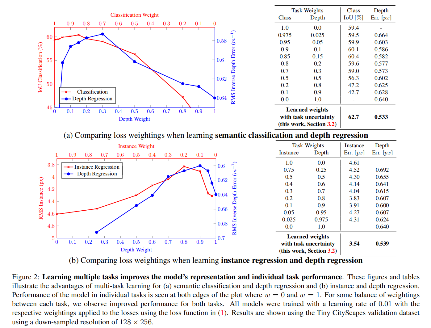
• task-independent uncertainty:
  $${\mathcal{L}}_{\text{total }}=\sum _i^M\sum _{j=\alpha ,\beta ,\gamma }{w}_j^i{\mathcal{L}}_j^i{\mathcal{L}}_{\text{total }}=\sum _i^M\sum _{j=\alpha ,\beta ,\gamma }\frac{1}{2}\left(\frac{1}{e^{s_j^i}}{\mathcal{L}}_j^i+s_j^i\right)$$

  Task-independent Uncertainty:

  Article: “Multi-Task Learning Using Uncertainty to Weigh Losses for Scene Geometry and Semantics”

  multi-task loss: ${\mathcal{L}}_{total}={\sum }_i{w}_i{\mathcal{L}}_i$

  Model performance is extremely sensitive to weight selection.

  

  In Bayesian modelling, there are two main types of uncertainty:

  • Epistemic⁴ uncertainty: Due to lack of training data.
  • Aleatoric⁵ uncertainty: Aleatoric uncertainty can be explained away with theability to observe all explanatory variables⁶ with increasing precision. It can be divided into:
    • Data-dependent (Heteroscedastic⁷ uncertainty): Depends on the input data.
    • Task-dependent (Homoscedastic⁸ uncertainty): It is a quantity which stays constant for all input data and varies between different tasks.

  Multi-task loss function based on maximising the Gaussian likelihood with homoscedastic uncertainty:

  • $f^W(x)\to$ output of a neural network with weights $W$ on input $x$
  • For regression task: $p\left(\mathbf{y}\mid {\mathbf{f}}^{\mathbf{W}}(\mathbf{x})\right)=\mathcal{N}\left({\mathbf{f}}^{\mathbf{W}}(\mathbf{x}),{\sigma }^2\right)$. The mean is given by the model out put.
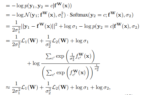
  • For classification task: $p(\mathbf{y}\mid {\mathbf{f}}^W(\mathbf{x})=\mathbf{softmax}({\mathbf{f}}^W(\mathbf{x}))$
  • In the case of multiple model outputs, we can factorise over the outputs: $p\left({\mathbf{y}}_1,\dots ,{\mathbf{y}}_K\mid {\mathbf{f}}^{\mathbf{W}}(\mathbf{x})\right)=p\left({\mathbf{y}}_1\mid {\mathbf{f}}^{\mathbf{W}}(\mathbf{x})\right)\dots p\left({\mathbf{y}}_K\mid {\mathbf{f}}^{\mathbf{W}}(\mathbf{x})\right)$. $y_n$ means outputs of different tasks.
  • Scaled version of Softmax: $p\left(\mathbf{y}\mid {\mathbf{f}}^{\mathbf{W}}(\mathbf{x}),\sigma \right)=\mathrm{Softmax}\left(\frac{1}{{\sigma }^2}{\mathbf{f}}^{\mathbf{W}}(\mathbf{x})\right)$
  • The log likelihood: $\log p\left(\mathbf{y}=c\mid {\mathbf{f}}^{\mathbf{W}}(\mathbf{x}),\sigma \right)=\frac{1}{{\sigma }^2}{f}_c^{\mathbf{W}}(\mathbf{x})-\log {\sum }_{c^{\prime }}\exp \left(\frac{1}{{\sigma }^2}{f}_{c^{\prime }}^{\mathbf{W}}(\mathbf{x})\right)$
  • 

3.6 Online Association

A tracklet is described with an appearance state $e_i$ and a motion state $m_i=(x,y,\gamma ,h,\dot{x},\dot{y},\dot{\gamma },\dot{h})$:

• $x,y$: bounding box center position
• $h$: bounding box height
• $\gamma$: bounding box ratio
• $\dot{x}$: velocity of $x$

For an incoming frame, compute motion affinity matrix $A_m$ and appearance affinity matrix $A_e$ using cosine similarity and Mahalanobis similarity respectively.

linear assignment:

• Hungarian algorithm:

(二)匈牙利算法简介_恒友成的博客-CSDN博客_匈牙利算法

• cost matrix: $C=\lambda A_e+(1-\lambda )A_m$

Matched $m_i$ is updated by Kalman filter, and $e_i$ is updated by $e_i^t=\alpha e_i^{t-1}+(1-\alpha )f_i^t$

Finally observations that are not assigned to any tracklets are initialized as new tracklets if they consecutively appear in 2 frames. A tracklet is terminated if it is not updated in the most current 30 frames.

---

---

1. /ˈpærədaɪm/ 典范 ↩︎

2. Separate Detection and Embedding ↩︎

3. Jointly learns the Detector and Embedding model. ↩︎

4. /ˌepɪˈstiːmɪk/ 认知的 ↩︎

5. /ˈeɪliətəri/ 偶然的 ↩︎

6. 解释性的变量 ↩︎

7. /hetərəusə’dæstik/ 异方差的 ↩︎

8. /həʊməʊskɪˈdæstɪk/ 同方差的 ↩︎