《Robotics, Vision and Control — Fundamental Algorithms in MATLAB》Chapter2. Exercies

1.Explore the effect of negative roll, pitch or yaw angles. Does transforming from RPY angles to rotation matrix then back to RPY angles give a different result to the starting value as it does for Euler angles?

fprintf('\n Question 1:\n');
f_origin=eye(3,3);
rpy=[-0.1,-0.2,0.3]
rpy2R = rpy2r(-0.1,-0.2, 0.3) % rpy-> R, 'XYZ'
R2rpy = tr2rpy(rpy2R)        %R -> rpy
trplot(f_origin,'color', 'r','frame','O');hold on;
trplot(rpy2R, 'color', 'g','frame','1');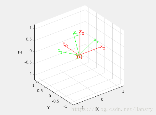

Answer:
As for Euler angles, we kown that mapping from rotation matrix to Euler angle is not unique. But there will not have multiple solutions from rotation matrix to roll-pitch-yaw angle, thanks to roll-pitch-yaw sequence allows all angles to have arbitrary sign. Unfortunately, roll-pitch-yaw has a singularity when $\theta_{p}= \pm \frac{\pi}{2}$ .

2.Explore the many options associated with trplot.

fprintf('\n Question 2:\n');
T_origin=eye(4,4);trplot(T_origin,'frame','O','color','red');hold on;  %define a identity matrix as the reference frame called {0}
T_A=T_origin*trotx(pi/4)*transl(0,0.5,0);  %rotate by 45 degress about the X axis, then a walk of 0.5 unit along the new y-axis 
trplot(T_A,'frame','A','color','g');  %frame{A}

T_B=T_origin*trotx(pi/4)*transl(-0.5,0,0);
trplot(T_B, 'frame', 'B', 'text_opts', {'FontSize', 10, 'FontWeight', 'bold'}); %change the parameter of text, frame{B}

T_C=T_origin*trotx(pi/4)*transl(0,0,0.4);
h = trplot(T_C, 'frame', 'C', 'color', 'y'); 
trplot(h, T_C);    %frame{C}
fprintf('\n The figure shows different result by changing the parameters of trplot \n')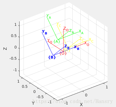

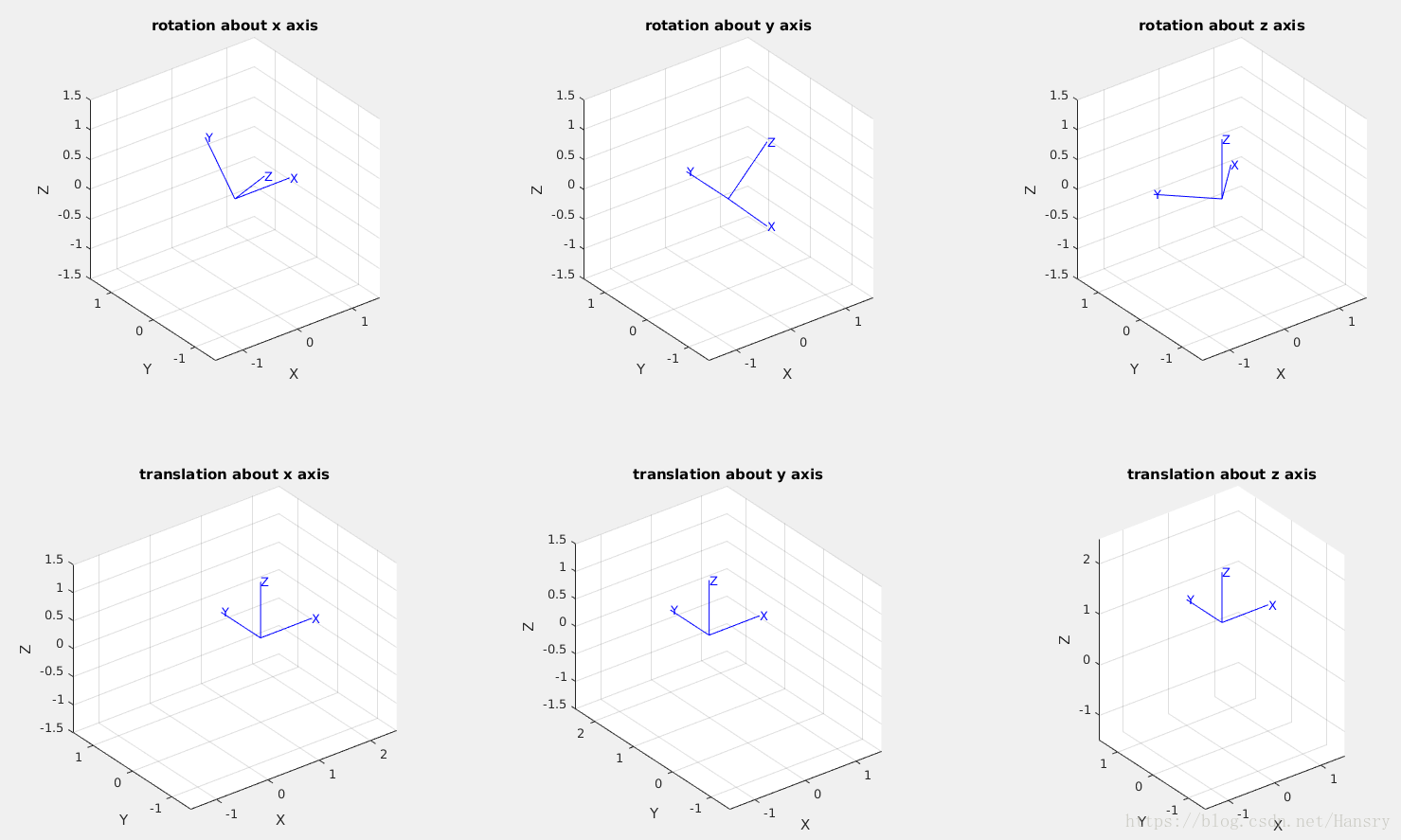
3.Use tranimate to show translation and rotational motion about various axes.

fprintf('\n Question 3:\n');
fprintf('\n The figure shows translation and rotational motion about various axes\n')
R_x=trotx(pi/4);  %Rotation
R_y=troty(pi/4);
R_z=trotz(pi/4);
subplot(231),title('rotation about x axis'),tranimate(R_x,'nsteps',20);
subplot(232),title('rotation about y axis'),tranimate(R_y,'nsteps',20);
subplot(233),title('rotation about z axis'),tranimate(R_z,'nsteps',20);

t_x=transl(1,0,0);  %translation
t_y=transl(0,1,0);
t_z=transl(0,0,1);
subplot(234),title('translation about x axis'),tranimate(t_x,'nsteps',20);
subplot(235),title('translation about y axis'),tranimate(t_y,'nsteps',20);
subplot(236),title('translation about z axis'),tranimate(t_z,'nsteps',20);

Running the code to see the motion of all the transformation.

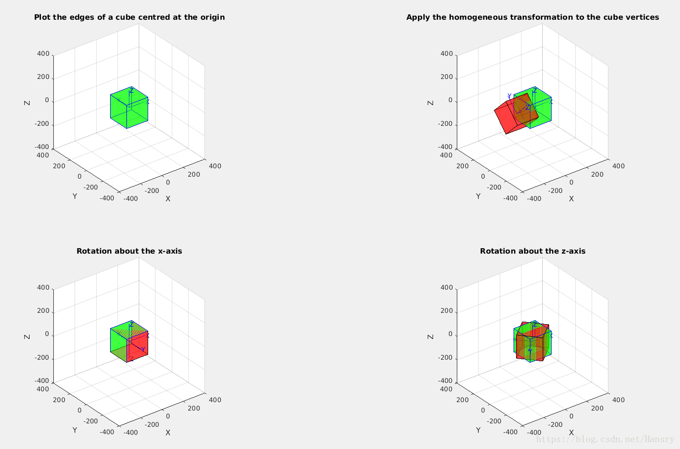
4. Animate a tumbling cube
a) Write a function to plot the edges of a cube centred at the origin.
b) Modify the function to accept an argument which is a homogeneous transformation which is applied to the cube vertices before plotting.
c) Animate rotation about the x-axis.
d) Animate rotation about all axes

plot_cube.m

function y=plot_cube(size,rotation_step,T_A)

origin=[0,0,0];   %To setup the origin of cube
x_orig= [0 1 1 0 0 0;                            %  -100   100   100  -100  -100  -100
    1 1 0 0 1 1;                                 %   100   100  -100  -100   100   100
    1 1 0 0 1 1;                                 %   100   100  -100  -100   100   100
    0 1 1 0 0 0];                                %   -100   100   100  -100  -100  -100
x_orig=(x_orig-0.5)*size+origin(1);              %  the x coordinate of all the cube vertices 

y_orig= [0 0 1 1 0 0;                              
    0 1 1 0 0 0;
    0 1 1 0 1 1;
    0 0 1 1 1 1];
y_orig=(y_orig-0.5)*size+origin(2);              % The same as the x_orig, but has different values

z_orig= [0 0 0 0 0 1;
    0 0 0 0 0 1;
    1 1 1 1 0 1;
    1 1 1 1 0 1];
z_orig=(z_orig-0.5)*size+origin(3);             % The same as the x_orig, but has different values

subplot(221);T_origin=eye(4,4);trplot(T_origin,'color','b','length',150);
title('Plot the edges of a cube centred at the origin');hold on;


%plot the edges of a cube centred at the origin
for i=1:6
    h=patch(x_orig(:,i),y_orig(:,i),z_orig(:,i),'g');  %Each face has four vertices and each cube has six faces,
    set(h,'edgecolor','b','facealpha',0.5);         % so the number of vertices we needed is 4x6=24
end
axis equal
axis([-400 400 -400 400 -400 400]);

%%Apply the homogeneous transformation to the cube vertices
x_t=x_orig;y_t=y_orig;z_t=z_orig;
subplot(222);title('Apply the homogeneous transformation to the cube vertices');
transformation_cube(false,rotation_step,'x',T_A,x_t,y_t,z_t); 

%%Rotation about the x-axis
x_r=x_orig;y_r=y_orig;z_r=z_orig;
subplot(223);title('Rotation about the x-axis');
transformation_cube(true,rotation_step,'x',T_A,x_r,y_r,z_r);

%%Rotation about the z-axis, here I can change the axis
x_r=x_orig;y_r=y_orig;z_r=z_orig;
subplot(224);title('Rotation about the z-axis');
transformation_cube(true,rotation_step,'z',T_A,x_r,y_r,z_r);

end


% First paparmeter: is it necessary to rotate? true or false
% rotation_setp: the step of rotation    
% 'x': ratate about which axis.
% T_A: the homogeneous matrix which applys to the transformation
% x_t,y_t,z_t: the cube vertices 
function transformation_cube(is_rotation,rotation_step,axes,T,x_orig,y_orig,z_orig)
    T_origin=eye(4,4);
    if is_rotation == false    
        rotation_step=pi/2;
    end

    for step=0:rotation_step:pi    
        x_r=x_orig;y_r=y_orig;z_r=z_orig;
        if is_rotation
            if axes=='x'
                T_tr=trotx(step);
            elseif axes=='y'
                T_tr=troty(step);
            elseif axes=='z'
                T_tr=trotz(step);
            end
        else
            T_tr=T;
        end

        for i=1:6
            for j=1:4
                point_t=[x_r(j,i),y_r(j,i),z_r(j,i)];point_t=point_t';
                point_hat=e2h(point_t);
                point_trans=h2e(T_tr*point_hat)';
                x_r(j,i)=point_trans(1);
                y_r(j,i)=point_trans(2);
                z_r(j,i)=point_trans(3);
            end
            q=patch(x_r(:,i),y_r(:,i),z_r(:,i),'r');
            set(q,'edgecolor','k','facealpha',0.5);
            p=patch(x_orig(:,i),y_orig(:,i),z_orig(:,i),'g');
            set(p,'edgecolor','b','facealpha',0.5);       
        end

        %subplot(plot_local);title('Rotation about the x-axis');
        R=T_tr*T_origin; 
        trplot(R,'color','b','length',150),trplot(T_origin,'color','b','length',150);hold on;
        axis equal
        axis([-400 400 -400 400 -400 400])  % set the range of each axis: x(-400,400), y(-400,400), z(-400,400)
        grid on; 
        if is_rotation
            getframe;    
            if step<pi-0.1  %To keep the last frame
                cla;
            end
        end
    end
end

fprintf('\n Question 4:\n');
fprintf('\n The figure shows translation and rotational motion of the cube about various axes\n')
size=200;   %the size of the cube edge
rotation_step=10*pi/180;  %the ratation setp of the cube 
T_A=trotx(pi/4)*transl(-150,0,0);
plot_cube(size,rotation_step,T_A);   % plot the edges of a cube centred at the origin.

Running the code to see the motion of all the transformation

5.Question Using Eq. 2.21 show that TT^{−1}=I.

fprintf('\n Question 5:\n');
T_5=trotx(pi/4)*troty(pi/4)*transl(0.3,0,0.3); % Here we define T as T_5.
trplot(T_origin,'frame','O','color','red');hold on;
T_1=T_5*T_origin;trplot(T_1,'frame','1','color','g');   

T_5_inv=inv(T_5);  %T_5_inv=T_5^{-1}
T_2= (T_5_inv)*T_1;trplot(T_2,'frame','2','color','b');  

%%%Answer:
% From the figure, we can see that  f_{1}=T_5*f_{0},
% f_{2}=T_5^{-1}*f_{1},so we get f_{2}=T_5^{-1}*T_5*f_{0} and f_{0}=f_{2},
% so here T_5^{-1}*T_5 = I
fprintf('\n The figure demostrates the equation TT^{−1}=I\n')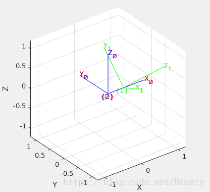

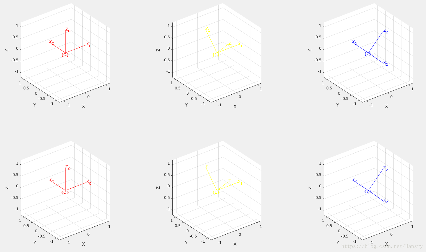
6.Generate the sequence of plots shown in Fig. 2.11

fprintf('\n Question 6:\n');
R=eye(3,3);subplot(231);trplot(R,'frame','O','color','red');hold on;
R_x1=rotx(pi/2);subplot(232);trplot(R_x,'frame','1','color','yellow');
R_y1=rotx(pi/2)*roty(pi/2);subplot(233);trplot(R_y,'frame','2','color','blue');

subplot(234);trplot(R,'frame','O','color','red');hold on;
R_x2=roty(pi/2);subplot(235);trplot(R_x,'frame','1','color','yellow');
R_y2=roty(pi/2)*rotx(pi/2);subplot(236);trplot(R_y,'frame','2','color','blue');

fprintf('\n The figure shows the sequence of plots shown in Fig. 2.11\n')

Answer:
Note that the different orders of rotation will produce the different results.

7.Where is Descarte’s skull?

fprintf('\n Question 7:\n');
fprintf('\nI do not konw the extactly meaning of this question, but literally, the  skull of Descarte is located in Museum of Man, Paris.\n');

8.Create a vector-quaternion class that supports composition, negation and point transformation.

VectorQuaternion.m （创建一个类）

classdef VectorQuaternion
   properties (SetAccess = private)  %set the inner variables as private
      vector
      Quaternion
   end

   methods
       function z=VectorQuaternion(q,t) %constructor
           z.vector=t;
           z.Quaternion=q;
       end

       function qp = plus(z1, z2)   %composition. See section 2.2.2, Page 36 and 37 of English version
            if isa(z1, 'VectorQuaternion') && isa(z2, 'VectorQuaternion') 
                qp.vector = z1.vector + z1.Quaternion*z2.vector;  %t_{1}+\dot{q}_{1}*t^{2}
                qp.Quaternion.s=z1.Quaternion.s*z2.Quaternion.s-dot(z1.Quaternion.v,z2.Quaternion.v); % s_{1}*s_{2}-v_{1}*v_{2}
                % s_{1}*v_{2}+s_{2}*v_{1}+v_{1}X v_{2}
                qp.Quaternion.v=z1.Quaternion.s*z2.Quaternion.v+z2.Quaternion.s*z1.Quaternion.v+cross(z1.Quaternion.v,z2.Quaternion.v);
            else 
                error('bad argument for function of VectorQuaternion');
            end
       end

       function q1=neg(z1)   %Negation.   
           if isa(z1, 'VectorQuaternion')
                q1.vector=(-1)*(inv(z1.Quaternion))*z1.vector;  % -\dot{q}^{-1}*t
                q1.Quaternion=inv(z1.Quaternion);  % \dot{q}^{-1}     
           else 
               error('bad argument for function of VectorQuaternion');
           end
       end

       function transform=vqtran(py,z2) %transformation for point
           if isa(z2, 'VectorQuaternion') && (length(py)==3)
                transform=z2.Quaternion*py+z2.vector;   %P_{x}=\dot{q}*P_{y}+t
           else
              error('unknown dimension of input or bad argument for function of VectorQuaternion')
           end
       end
     end
end

fprintf('\n Question 8:\n');
point3f=[1.0,1.5,2.0]';   

fprintf('\n Declare two VectorQuaternion type variables:\n')
quant1=Quaternion(rpy2tr(0.1,0.2,0.3));t1=[0,0.4,0.4]';   
quant2=Quaternion(rpy2tr(0.0,0.2,0.3));t2=[0.4,0,0.4]';  

VectorQuaternion1=VectorQuaternion(quant1,t1)   %VectorQuanternion(q,t), where q is a quaternion type variable,
VectorQuaternion2=VectorQuaternion(quant2,t2)   %while t is a 3x1 vector .

fprintf('\n Composite quant1 and quant2:\n');
composition=plus(VectorQuaternion1,VectorQuaternion2) %VectorQuaternion1+VectorQuaternion2

fprintf('\n Negation of quant1 and quant2:\n');
negation1=neg(VectorQuaternion1)  % neg(vq) %where vq is a VectorQuaternion type variable
negation2=neg(VectorQuaternion2) 

fprintf('\n Point transformation of quant1 and quant2\n')
p_t1=vqtran(point3f,VectorQuaternion1)  % vqtran(p,vq) where p is a point3f(3x1 vector) avaliable, vq is a VetctorQuaternion
p_t2=vqtran(point3f,VectorQuaternion2)  % avariable, which indicts the transformation.

Result：

 Declare two VectorQuaternion type variables:

VectorQuaternion1 = 

  VectorQuaternion with properties:

        vector: [3x1 double]
    Quaternion: [1x1 Quaternion]


VectorQuaternion2 = 

  VectorQuaternion with properties:

        vector: [3x1 double]
    Quaternion: [1x1 Quaternion]


 Composite quant1 and quant2:

composition = 

        vector: [3x1 double]
    Quaternion: [1x1 struct]


 Negation of quant1 and quant2:

negation1 = 

        vector: [3x1 double]
    Quaternion: [1x1 Quaternion]


negation2 = 

        vector: [3x1 double]
    Quaternion: [1x1 Quaternion]


 Point transformation of quant1 and quant2

p_t1 =

    0.8992
    1.9344
    2.4217


p_t2 =

    1.2992
    1.7285
    2.2584

上述答案为根据自己对该章知识的学习以及总结，可能存在不足的地方，希望各位博友能够指出问题，谢谢！