2.For a lspb trajectory from 0 to 1 in 50 steps explore the effects of specifying the velocity for the constant velocity segment. What are the minimum and maximum bounds possible?
%Code:
[s1,sd1,sdd1]=lspb(0,1,50,0.025);
[s2,sd2,sdd2]=lspb(0,1,50,0.03);
[s3,sd3,sdd3]=lspb(0,1,50,0.035);
[s4,sd4,sdd4]=lspb(0,1,50,0.04);
plot(sd1,'r'),hold on,plot(sd2,'g'),plot(sd3,'b'),plot(sd4,'y'),grid on;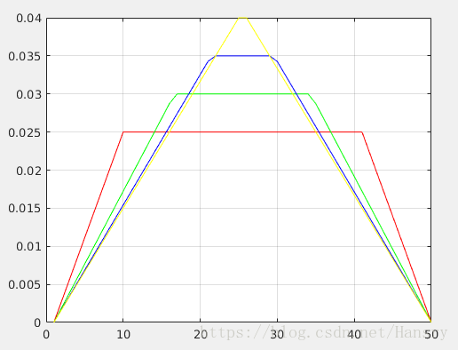
Answer:
1. [s,sd,sdd] = lspb(q0, q1, t, V), where q0=0, q1=1,t=50, tf=max(0:t-1) and abs(q1-q0)/tf <= abs(V) <= 2*abs(q1-q0)/tf
   in this question, tf=49, so we have 0.020408 <= abs(V) <= 0.040816.

2. The constant velocity segment is descrease along with the increasing of the specific velocity.
   The minimum and maximum value of the specific velocity are 0.020408 and 0.040816 respectively.
3.For a trajectory from 0 to 1 and given a maximum possible velocity of 0.025 compare how many time steps are required for each of the tpoly and lspb trajectories?
fprintf('\nFor lspb() function, 41<= time_steps <=81; for tpoly() function, time_steps=76\n')Answer:
For lspb function, from question2, we know that abs(q1-q0)/tf <= abs(V) <= 2*abs(q1-q0)/tf.
In this function, abs(V)=0.025, so we get 40 <= tf<= 80, and 41<= time_steps <= 81.
For tpoly function, the solution is as following:
1. |q0 | |0, 0, 0, 0, 0, 1| |A|
|qf | |tf^5, tf^4, tf^3, tf^2, tf, 1| |B|
|qd0|= |0, 0, 0, 0, 1, 0|*|C|
|qdf| |5*tf^4, 4*tf^3, 3*tf^2, 2*tf, 1, 0| |D|
| 0 | |0, 0, 0, 2, 0, 0| |E|
| 0 | |20*tf^3, 12*tf^2, 6*tf, 2, 0, 0| |F|, where qf=1, q0=qd0=qdf=0
2. |A| |-6/tf^5, 6/tf^5, -3/tf^4, -3/tf^4, -1/(2*tf^3), 1/(2*tf^3) | |0| | 6/tf^5 |
|B| |15/tf^4, -15/tf^4, 8/tf^3, 7/tf^3, 3/(2*tf^2), -1/tf^2 | |1| |-15/tf^4|
|C|= |-10/tf^3, 10/tf^3, -6/tf^2, -4/tf^2, -3/(2*tf), 1/(2*tf)|*|0|=|10/tf^3 |
|D| | 0, 0, 0, 0, 1/2, 0 | |0| | 0 |
|E| | 0, 0, 1, 0, 0, 0 | |0| | 0 |
|F| | 1, 0, 0, 0, 0, 0 | |0| | 0 |
3. Velocity=(30/tf^5)*t^4 + (-60/tf^4)*t^3 + (30/tf^3)*t^2 ...(1)
when t=tf/2, we have maximum velocity, which equals to 0.025.
4. In equation (1), we replace t by tf/2, and get tf=75, so the time_steps equals to tf+1=76.4.Use tranimate to compare rotational interpolation using quaternions, Euler anglesand roll-pitch-yaw angles. Hint: use the quaternion interp method, and mtraj with tr2eul and eul2tr
a) Use mtraj to interpolate Euler angles between two orientations and display the rotating frame using tranimate.
%Code:
close all;
R0=rotz(-1)*roty(-1); %Define two orientations
R1=rotz(1)*roty(1);

rpy0=tr2rpy(R0);rpy1=tr2rpy(R1); %Define two rpy angles
rpy=mtraj(@tpoly,rpy0,rpy1,50);  %roll-pitch-yaw
subplot(131),title('Interpolation using roll-pitch-yaw angles'),tranimate(rpy2tr(rpy));

q0=Quaternion(R0);  %Define two quaternions
q1=Quaternion(R1);
q=interp(q0,q1,[0:49]'/49);
subplot(132),title('Interpolation using quaternions'),tranimate(q);

eul0=tr2eul(R0);
eul1=tr2eul(R1);
eul=mtraj(@tpoly,eul0,eul1,50);
subplot(133),title('Interpolation using euler angles'),tranimate(eul2tr(eul));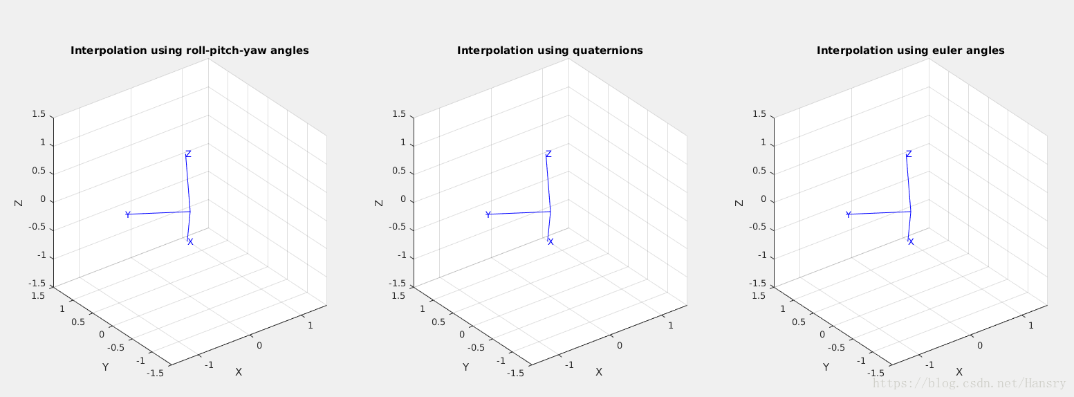
Answer:
The figure shows the animate of the rotational interpolation using quaternions, Euler angles
and roll-pitch-yaw angles. The quaternions is the best one to achieve rotational interpolation
b) Repeat for the case choose where the final orientation is at a singularity. What happens?
%Code:
close all;
R0 =rotz(pi/3)*roty(pi/6);  %Initial start point and .
R1 = rotx(pi/3)*roty(pi/2); %Singularity end point

q0=Quaternion(R0); %Quaternion conversion
q1=Quaternion(R1);
qm = interp(q0,q1,0.5);
q = interp(q0,q1,[0:49]'/49);
subplot(331),title('Start point using quaternion'),plot(q0); %start point
subplot(332),title('End point using quaternion'),plot(q1); %end point
subplot(333),title('Tranimate using quaternion'),tranimate(q); %tranimate respectively

rpy0 = tr2rpy(R0); %rpy conversion
rpy1=tr2rpy(R1);
rpy = mtraj(@tpoly, rpy0 ,rpy1 , 50);
subplot(334),title('Start point using rpy'),trplot(rpy2tr(rpy0));
subplot(335),title('End point using rpy'),trplot(rpy2tr(rpy1));
subplot(336),title('Tranimate using rpy'),tranimate(rpy2tr(rpy));

eul0 = tr2eul(R0); %Eular conversion
eul1 = tr2eul(R1);
eul = mtraj(@tpoly, eul0 , eul1 ,50);
subplot(337),title('Start point using eular'),trplot(eul2tr(eul0));
subplot(338),title('End point using eular'),trplot(eul2tr(eul1));
subplot(339),title('Tranimate using eular'),tranimate(eul2tr(eul));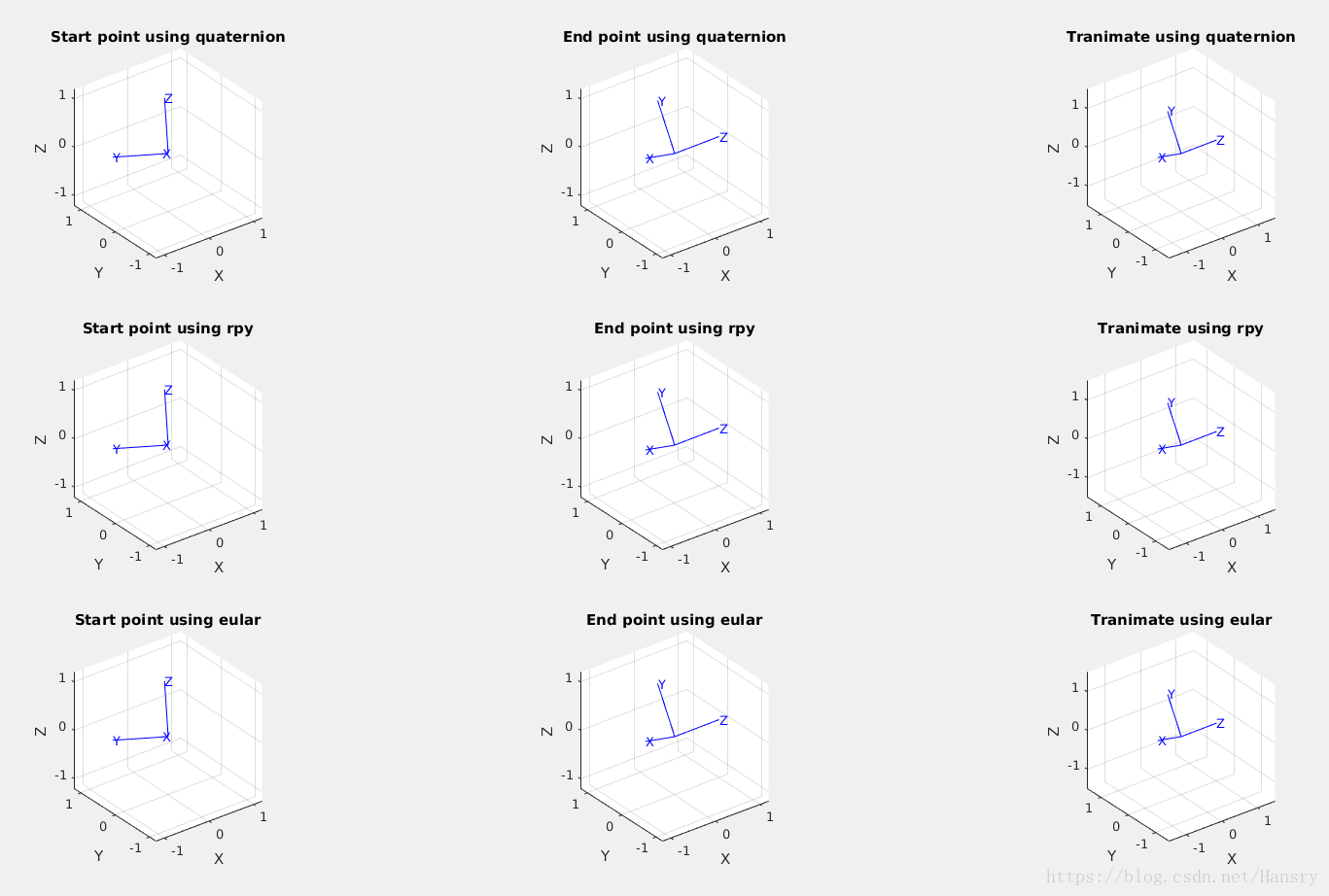
Answer:
Though the final orientation is at a singularity, there is nothing different when repeat for the case.
5.Repeat for the case where the interpolation passes through a singularity. What happens?
%Code
close all;
R0 =rotz(pi/3)*roty(pi/6);  %Initial start point and .
R1 = rotx(pi/3)*roty(pi/2); %Singularity state point
R2 = rotx(pi/3)*roty(pi/6); %End point
rpy0=tr2rpy(R0);rpy1=tr2rpy(R1);rpy2=tr2rpy(R2);
rpy_former = mtraj(@tpoly, rpy0 ,rpy1 , 50);
rpy_later = mtraj(@tpoly, rpy1 ,rpy2 , 50);
rpy=[rpy_former;rpy_later];
tranimate(rpy2tr(rpy));
Answer:
we use roll-pitch-yaw angles to show the situation where the interpolation
passes through a singularity. When repeat for the case, there are two
problems: 1. The trajectory is not unique anymore beacause of the
singularity state. 2.The trajectory is discontinuity. In general, we have
better use quaternion to represent the rotation.6.Develop a method to quantitatively compare the performance of the different orientation interpolation methods.
%Code:
close all;
Point_z=[0,0,1,1]';
R_origin=eye(3,3);trplot(R_origin,'frame','O','color','red',{'FontSize',10, 'FontWeight', 'bold'});hold on;
draw_sphere();
R0=eye(3,3);
R1=rotz(1)*roty(1);trplot(R1,'frame','D','color','b',{'FontSize', 10, 'FontWeight', 'bold'});
rpy0=tr2rpy(R0);rpy1=tr2rpy(R1);
rpy=mtraj(@tpoly,rpy0,rpy1,50);
%tranimate(rpy2tr(rpy));
for i=1:50
    Point=rpy2tr(rpy(i,:))*Point_z;
    p1=Point(1);p2=Point(2);p3=Point(3);
    plot3(p1,p2,p3, 'r*'),hold on;  %'Red' represents rotational interpolation using rpy angles
end

eul0=tr2eul(R0);
eul1=tr2eul(R1);
eul=mtraj(@tpoly,eul0,eul1,50);
for i=1:50
    Point=eul2tr(eul(i,:))*Point_z;
    p1=Point(1);p2=Point(2);p3=Point(3);
    plot3(p1,p2,p3, 'y*'),hold on;  %'yellow' represents rotational interpolation using eular angles
end

q0=Quaternion(R0);
q1=Quaternion(R1);
q=interp(q0,q1,[0:49]'/49);
for i=1:50
    Point=q(i).R*Point_z(1:3);
    p1=Point(1);p2=Point(2);p3=Point(3);
    plot3(p1,p2,p3, 'b*'),hold on;  %'blue' represents rotational interpolation using quaternion
end
fprintf('\n  yellow : using eular angles; blue : using quaternion; red : using rpy angles \n')
%draw_sphere.m
function draw_sphere()
t=linspace(0,pi,25);
p=linspace(0,2*pi,25);
[theta,phi]=meshgrid(t,p);
x=sin(theta).*sin(phi);
y=sin(theta).*cos(phi);
z=cos(theta);
surf(x,y,z);
axis equal;
alpha(0.6);
axis on;
end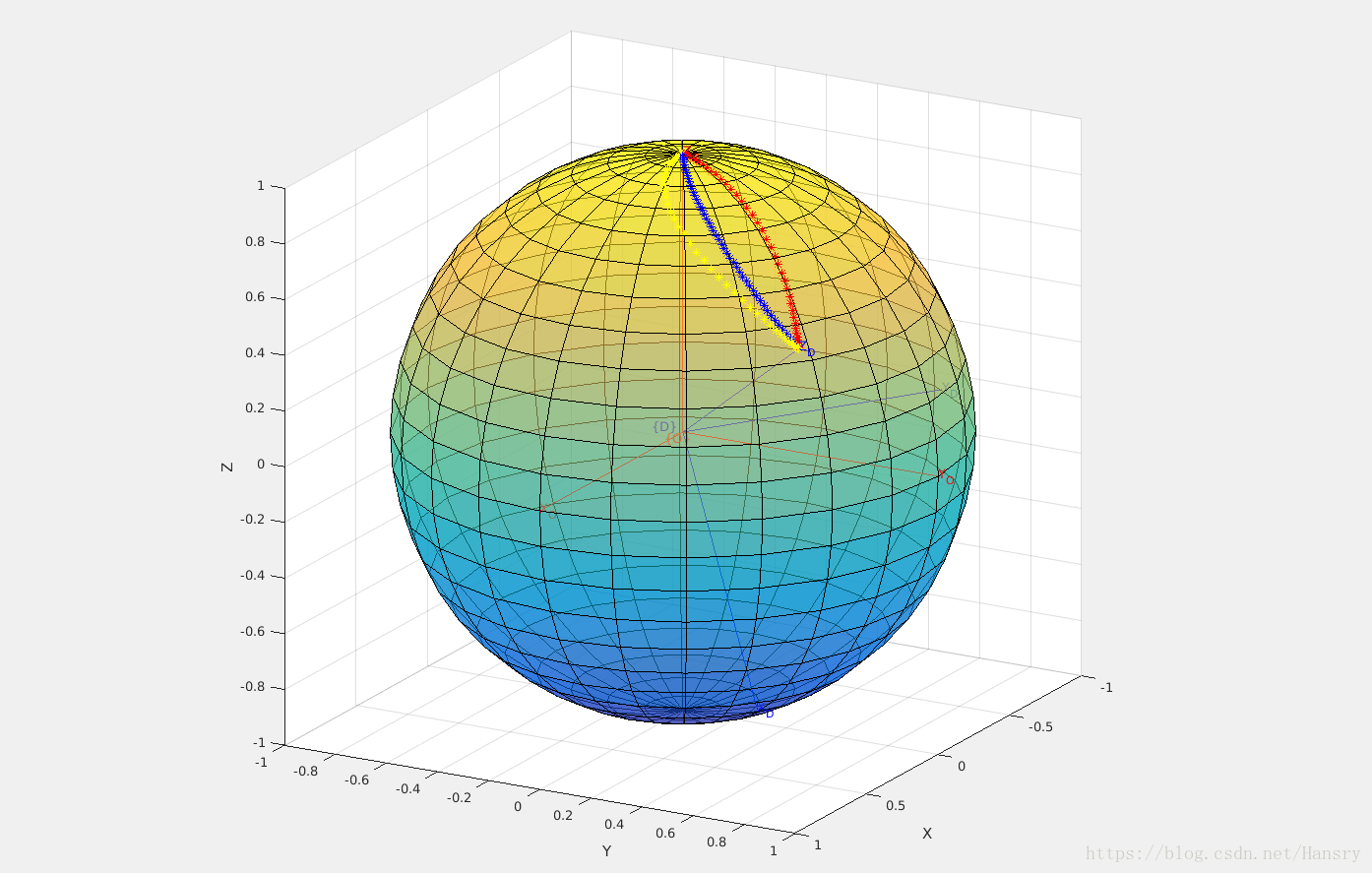
Answer:
From the figure, we can explicity see the trajectories of these three methods and the red, blue, yellow
colors are representing using rpy angles, using eular angles, using quaternion respectively.
Through this way, we would easily evaluate the trajectory, the velocity of these three method.
7.For the mstraj example (page 47)
a) Repeat with different initial and final velocity.

%Code
close all;
via=[4,1; 4,4; 5,2; 2,5];
q_tran=mstraj(via,[2,1],[],[4,1],0.05,0.5,[1,1],[2,2]); %initial and end velocity are [0.025,0.025] and [0,0] respectively
plot(q_tran,'--'),grid on,hold on;
q_tran1=mstraj(via,[2,1],[],[4,1],0.05,0.5,[0,0],[2,2]);%initial and end velocity are [0,0] and [0.025,0.025] respectively
plot(q_tran1,'o');
q_tran2=mstraj(via,[2,1],[],[4,1],0.05,0.5,[1,1],[1,1]); %initial and end velocity are [0,0] and [0,0] respectively
plot(q_tran2,'h');
title('The effect of different initial velocity and end velocity');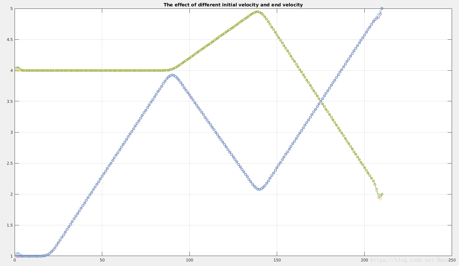
Answer:
Two condition:
1.when two trajectories have the same initial velocity, the trajectory has
a sharper end which end velocity is larger.

2.when two trajectories have the same end velocity, the trajectory has a sharper
start which initial velocity has a larger.

Please pay attention to the initial state and end state of those trajectories.
%}
b) Investigate the effect of increasing the acceleration time. Plot total time as a function of acceleration time.
%Code:
close all;
via=[4,1; 4,4; 5,2; 2,5];
q=mstraj(via,[2,1],[],[4,1],0.05,0);
subplot(121);plot(q,'--'),grid on, hold on;
q1=mstraj(via,[2,1],[],[4,1],0.05,0.5);
subplot(121);plot(q1,'-');
q2=mstraj(via,[2,1],[],[4,1],0.05,1);
subplot(121);plot(q2,'h');
title('The effect of increasing the acceleration time');
xlabel('Time')
ylabel('Distance')
legend('acc-time_0=0','acc-time_1=0','acc-time_0=0.5','acc-time_1=0.5','acc-time_0=1','acc-time_1=1','Location','SouthEast');

sum_time=0:0.02:3;
acc_time=0:0.02:3;
count=1;
for i=0:0.02:3
   time_q=mstraj(via,[2,1],[],[4,1],0.05,i);
   sum_time(count)=length(time_q);
   acc_time(count)=i;
   count=count+1;
end
subplot(122);plot(acc_time,sum_time,'-'),grid on;
xlabel('Acceleration time')
ylabel('Total time')
title('Total time as the function of acceleration time')
Answer:
Along with the incresing of the acceleration time, the trajectory of both
axis become more smooth which also means that the trajectory takes more
time to complete.

The graph of tatal time as the function of acceleration time are showed
above.
上述答案为根据自己对该章知识的学习以及总结,可能存在不足的地方,希望各位博友能够指出问题。