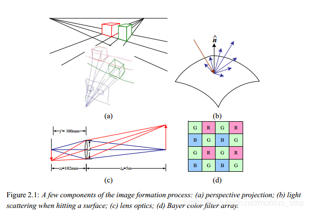
Computer Vision: Algorithms and Applications - Chapter 2 Image formation (1)

在这里插入图片描述

2.1 Geometric image formation

In this section, I introduce the basic 2D and 3D primitives used in this textbook, namely points, lines, and planes. I also describe how 3D features are projected into 2D features. More detailed descriptions of these topics (along with a gentler and more intuitive introduction) can be found in textbooks on multiple-view geometry (Hartley and Zisserman 2000, Faugeras and Luong 2001).

2.1.1 Geometric primitives

Geometric primitives form the basic building blocks used to describe three-dimensional shape. In this section, I introduce points, lines, and planes. Later sections of the book cover curves (§4.4 and §11.2), surfaces (§11.5), and volumes (§11.3).

2D Points. 2D Points (pixel coordinates in an image) can be denoted using a pair of values, $\boldsymbol {x} = (x, y) \in R^2$ , or alternatively
$\boldsymbol x = \begin{bmatrix} x \\ y \end{bmatrix}$
(As stated in the introduction, we use the $(x_1, x_2, ...)$ notation to denote column vectors.)
2D points can also be represented using homogeneous coordinates, $\tilde{\boldsymbol x} = (x, y, w) \in P^2$ , where vectors that differ only by scale are considered to be equivalent. $P^2 = R^3 − (0, 0, 0)$ is called the 2D projective space.

A homogeneous vector $\tilde{\boldsymbol x}$ can be converted back into an inhomogeneous vector $\boldsymbol x$ by dividing through by the last element $w$ , i.e.,
$\tilde{\boldsymbol x} = (x, y, w) = w(x, y, 1) = w \bar{\boldsymbol x}$
where $\bar x = (x, y, 1)$ is the augmented vector. Homogeneous points whose last element is $w = 0$ are called ideal points or points at infinity and do not have and equivalent inhomogeneous representation.

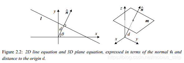
2D Lines. 2D lines can also be represented using homogeneous coordinates $\tilde{\boldsymbol l} = (a, b, c)$ . The corresponding line equation is
$\bar{\boldsymbol x} \cdot \bar{\boldsymbol l} = ax + by + c = 0$
We can normalize the line equation vector so that $\boldsymbol l = (n_x, n_y, d) = (\hat{\boldsymbol n}, d)$ with $\Vert \hat{\boldsymbol n}\Vert = 1$ . In this case, $\hat{\boldsymbol n}$ is the normal vector perpendicular to the line, and $d$ is its distance to the origin (Figure 2.2). (The one exception to this normalization is the line at infinity $\bar{\boldsymbol l} = (0, 0, 1)$ , which includes all (ideal) points at infinity.)
在这里插入图片描述
We can also express $KaTeX parse error: Expected '}', got 'EOF' at end of input: …t{\boldsymbol n$ as a function of rotation angle $θ,\hat{\boldsymbol n} = (n_x, n_y) = (cos θ, sin θ)$ (Figure 2.2). This representation is commonly used in the Hough transform line finding algorithm, which is discussed in §4.3.2. The combination $(θ, d)$ is also known as polar coordinates.

When using homogeneous coordinates, we can compute the intersection of two lines as
$\tilde{\boldsymbol x} = \tilde{\boldsymbol l}_1 × \tilde{\boldsymbol l}_2$
where $×$ is the cross-product operator. Similarly, the line joining two points can be written as
$\tilde{\boldsymbol l} = \tilde{\boldsymbol x}_1 × \tilde{\boldsymbol x}_2$

When trying to fit an intersection point to multiple lines, or conversely a line to multiple points, least square techniques (§5.1.1 and Appendix A.2) can be used, as discussed in Exercise 2.1.

2D Conics. There are also other algebraic curves that can be expressed with simple polynomial homogeneous equations. For example, the conic sections (so called because they arise as the intersection of a plane and a 3D cone) can be written using a quadric equation
$\tilde{\boldsymbol x}^T\boldsymbol Q \tilde{\boldsymbol x} = 0$
These play useful roles in the study of multi-view geometry and camera calibration (Hartley and Zisserman 2000, Faugeras and Luong 2001) but are not used extensively in this book.

3D Points. Point coordinates in three dimensions can be written using inhomogeneous coordinates $\boldsymbol x = (x, y, z) \in R^3$ or homogeneous coordinates $\tilde{\boldsymbol x} = (x, y, z, w) \in P^3$ . As before, it is sometimes useful to denote a 3D point using the augmented vector $\bar{\boldsymbol x} = (x, y, z, 1)$ with $\tilde{\boldsymbol x} = w \bar{\boldsymbol x}$ .

[ Note: In the “Note on notation” section of the intro, I said that we would use $p$ for 3D points. What do we want to do? Move between the two, as convenient? Is there any problem using $\boldsymbol x$ for points, since $\boldsymbol x$ looks so similar to $x$ ? ]
在这里插入图片描述

3D Planes. 3D planes can also be represented as homogeneous coordinates $\tilde{\boldsymbol m} = (a, b, c, d)$ with a corresponding plane equation
$\bar{\boldsymbol x} \cdot \tilde{\boldsymbol m} = ax + by + cz + d = 0$

We can also normalize the plane equation as $\boldsymbol m = (n_x, n_y, n_z, d) = (\hat{\boldsymbol n}, d)$ with $\hat{\boldsymbol n} = 1$ .
In this case $\hat{\boldsymbol n}$ is the normal vector perpendicular to the plane, and d is its distance to the origin (Figure 2.2). As with the case of 2D lines, the plane at infinity $\tilde{\boldsymbol m} = (0, 0, 0, 1)$ , which contains all the points at infinity, cannot be normalized (i.e., it does not have a unique normal, nor does it have
a finite distance).

We can express $\hat{\boldsymbol n}$ as a function of two angles $(θ, φ)$ , $\hat{\boldsymbol n} = (cos θ cos φ, sin θ cos φ, sin φ)$ , i.e., using spherical coordinates, but these are less commonly used than polar coordinates since they do not uniformly sample the space of possible normal vectors.

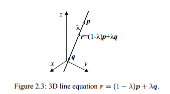
3D Lines. Lines in 3D are less elegant than either lines in 2D or planes in 3D. One possible representation is to use two points on the line, $(\boldsymbol p, \boldsymbol q)$ . Any other point on the line can be expressed as a linear combination of these two points
$\boldsymbol r = (1 − λ)\boldsymbol p + λ\boldsymbol q, (2.8)$
as shown in Figure 2.3. If we restrict $0 ≤ λ ≤ 1$ , we get the line segment joining $p$ and $q$ .

If we use homogeneous coordinates, we can write the line as
$\tilde{\boldsymbol r} = µ\tilde{\boldsymbol p} + λ\tilde{\boldsymbol q}$
A special case of this is when the second point is at infinity, i.e., $\tilde{\boldsymbol q} = (d_x, d_y, d_z, 0) = (\hat{\boldsymbol d} , 0)$ . Here, we see that $\hat{\boldsymbol d}$ is the direction of the line. We can then re-write the inhomogeneous 3D line equation as
$\boldsymbol r = \boldsymbol p + λ\hat{\boldsymbol d}$
A disadvantage of the endpoint representation for 3D lines is that it has too many degrees of freedom: 6 (3 for each endpoint), instead of the 4 degrees that a 3D line truly has. However, if we fix the two points on line to lie in specific planes, we obtain a 4 d.o.f. representation. For example, if we are representing nearly vertical lines, then $z = 0$ and $z = 1$ form two suitable planes, i.e., the $(x, y)$ coordinates in both planes provide the 4 coordinates describing the line. This kind of two-plane parameterization is used in the Lightfield and Lumigraph image-based rendering systems described in §12 to represent the collection of rays seen by a camera as it moves in front of an object. The two endpoint representation is also useful for representing line segments, even when their exact endpoints cannot be seen (only guessed at).

If we wish to represent all possible lines without bias towards any particular orientation, we can use Plucker coordinates (Hartley and Zisserman 2000, Chapter 2)(Faugeras and Luong 2001, Chapter 3). These coordinates are the six independent non-zero entries in the 4×4 skew symmetric matrix
$L = \tilde{\boldsymbol p}\tilde{\boldsymbol q}^T − \tilde{\boldsymbol q}\tilde{\boldsymbol p}^T$
where p˜and q˜are any two (non-identical) points on the line. This representation has only 4 degrees of freedom, since $L$ is homogeneous and also satisfies $det(L) = 0$ (which results in a quadratic constraint on the Plucker coordinates).

In practice, I find that in most applications, the minimal representation is not essential. An adequate model of 3D lines can be obtained by estimating their direction (which may be known ahead of time, e.g., for architecture) and some point within the visible portion of the line (e.g., see §6.5.1), or by using the two endpoints, since lines are most often visible as finite line segments. However, if you are interested in more details about the topic of minimal line parameterizations, Forstner (2005) discusses various ways to infer and model 3D lines in projective geometry, as well as how to estimate the uncertainty in such fitted models.

3D Quadrics. The 3D analogue to conic sections are quadric surfaces
$\bar{\boldsymbol x}^TQ\bar{\boldsymbol x} = 0$
(Hartley and Zisserman 2000, Chapter 2). Again, while these are useful in the study of multi-view geometry and can also serve as useful modeling primitives (spheres, ellipsoids, cylinders), we do not study them in great detail in this book.

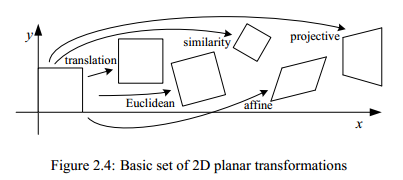
2.1.2 2D transformations

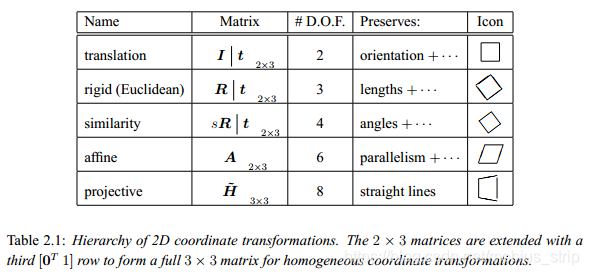
Having defined our basic primitives, we can now turn our attention to how they can be transformed. The simplest transformations occur in the 2D plane and are illustrated in Figure 2.4.
在这里插入图片描述
Translation. 2D translations can be written as $x' = x + t$ or
$\boldsymbol x' = \begin{bmatrix} \boldsymbol I & \boldsymbol t \end{bmatrix} \bar{\boldsymbol x}$
where $\boldsymbol I$ is the (2 × 2) identity matrix or
$\bar{\boldsymbol x}' = \begin{bmatrix} \boldsymbol I & \boldsymbol t \\ \boldsymbol 0^T & 1 \end{bmatrix} \bar{\boldsymbol x}$
where $\boldsymbol 0$ is the zero vector. Using a 2 × 3 matrix results in a more compact notation, whereas using a full-rank 3 × 3 matrix (which can be obtained from the 2 × 3 matrix by appending a $\begin{bmatrix} \boldsymbol 0^T & 1 \end{bmatrix}$ row) makes it possible to chain transformations together using matrix multiplication. Note that in any equation where an augmented vector such as x¯ appears on both sides, it can always be replaced with a full homogeneous vector $\tilde{\boldsymbol x}$ .

Rotation + translation. This transformation is also known as 2D rigid body motion or the 2D Euclidean transformation (since Euclidean distances are preserved). It can be written as $\boldsymbol x' = \boldsymbol R \boldsymbol x + \boldsymbol t$ or
$\boldsymbol x' = \begin{bmatrix} \boldsymbol R & \boldsymbol t \end{bmatrix} \bar{\boldsymbol x}$
where
$\boldsymbol R = \begin{bmatrix} cos θ & − sin θ \\ sin θ & cos θ \end{bmatrix}$
is an orthonormal rotation matrix with $\boldsymbol R \boldsymbol R^T = \boldsymbol I$ and $\Vert \boldsymbol R \Vert = 1$ .

Scaled rotation. Also known as the similarity transform, this transform can be expressed as $\boldsymbol x' = s\boldsymbol R \boldsymbol x + \boldsymbol t$ where s is an arbitrary scale factor. It can also be written as
$\boldsymbol x' = \begin{bmatrix} s\boldsymbol R & \boldsymbol t \end{bmatrix} \bar{\boldsymbol x} = \begin{bmatrix} a & −b & t_x \\ b & a & t_y \end{bmatrix} \bar{\boldsymbol x}$
where we no longer require that $a^2 + b^2 = 1$ . The similarity transform preserves angles between lines.
在这里插入图片描述
Affine. The affine transform is written as $\boldsymbol x' = A \bar{ \boldsymbol x}$ , where $\boldsymbol A$ is an arbitrary 2 × 3 matrix, i.e.,
$\boldsymbol x' = \begin{bmatrix} a_{00} & a_{01} & a_{02} \\ a_{10} & a_{11} & a_{12} \end{bmatrix} \bar{\boldsymbol x}$
Parallel lines remain parallel under affine transformations.

Projective. This transform, also known as a perspective transform or homography, operates on homogeneous coordinates,
$\tilde{\boldsymbol x}' = \tilde{\boldsymbol H} \tilde{\boldsymbol x},$
where $\tilde{\boldsymbol H}$ is an arbitrary 3 × 3 matrix. Note that $\tilde{\boldsymbol H}$ is itself homogeneous, i.e., it is only defined up to a scale, and that two $\tilde{\boldsymbol H}$ matrices that differ only by scale are equivalent. The resulting homogeneous coordinate $\tilde{\boldsymbol x}'$ must be normalized in order to obtain an inhomogeneous result $\boldsymbol x$ , i.e.,
$x' = \frac{ h_{00}x + h_{01}y + h_{02} }{h_{20}x + h_{21}y + h_{22} } and y' = \frac{ h_{10}x + h_{11}y + h_{12} }{h_{20}x + h_{21}y + h_{22} }$
Perspective transformations preserve straight lines (i.e., they remain straight after the transformation).

Hierarchy of 2D transformations. The preceding set of transformations are illustrated in Figure 2.4 and summarized in Table 2.1. The easiest way to think of these is as a set of (potentially restricted) 3×3 matrices operating on 2D homogeneous coordinate vectors. Hartley and Zisserman (2000) contains a more detailed description of the hierarchy of 2D planar transformations.

The above transformations form a nested set of groups, i.e., they are closed under composition and have an inverse that is a member of the same group. (This will be important later when applying these transformations to images in §3.5.) Each (simpler) group is a subset of the more complex group below it.

Co-vectors. While the above transformations can used to transform points in a 2D plane, can they also be used directly to transform a line equation? Consider the homogeneous equation $\tilde{\boldsymbol l} \cdot \tilde{\boldsymbol x} = 0$ .
If we transform $\tilde{\boldsymbol x}' = \tilde{\boldsymbol H} \boldsymbol x= 0$ , we obtain
$\tilde{\boldsymbol l}' \cdot \tilde{\boldsymbol x}' = \tilde{\boldsymbol l}^T \tilde{\boldsymbol H} \tilde{\boldsymbol x} = (\tilde{\boldsymbol H}^T \tilde{\boldsymbol l})^T\tilde{\boldsymbol x} = \tilde{\boldsymbol l} \cdot \tilde{\boldsymbol x} = 0$
i.e., $\tilde{\boldsymbol l}' = \tilde{\boldsymbol H}^{-T} \tilde{\boldsymbol l}$ . Thus, the action of a projective transformation on a co-vector such as a 2D line or 3D normal can be represented by the transposed inverse of the matrix, which is equivalent to the adjoint of $\tilde{\boldsymbol H}$ , since projective transformation matrices are homogeneous. Jim Blinn’s (1998) book Dirty Pixels contains two chapters (9 and 10) describing the ins and outs of notating and manipulating co-vectors.

Additional transformations.

While the above transformations are the ones we use most extensively, a number of additional transformations are sometimes used.

Stretch/squash. This transformation changes the aspect ratio of an image,
$x' = s_xx + t_x \\ y' = s_yy + t_y,$
and is a restricted form of an affine transformation. Unfortunately, it does not nest cleanly with the groups listed in Table 2.1.
Planar surface flow. This 8-parameter transformation (Horn 1986, Bergen et al. 1992, Girod et al. 2000),
$x' = a_0 + a_1x + a_2y + a_6x^2 + a_7xy \\ y' = a_3 + a_4x + a_5y + a_7x^2 + a_6xy,$
arises when a planar surface undergoes a small 3D motion. It can thus be thought of as a small motion approximation to a full homography. Its main attraction is that it is linear in the motion parameters $a_k$ , which are often the quantities being estimated.
在这里插入图片描述
Bilinear interpolant. This 8-parameter transform (Wolberg 1990),
$x' = a_0 + a_1x + a_2y + a_6xy \\ y' = a_3 + a_4x + a_5y + a_7xy,$
can be used to interpolate the deformation due to the motion of the four corner points of a square. (In fact, it can interpolate the motion of any four non-colinear points.) While the deformation is linear in the motion parameters, it does not generally preserve straight lines (only lines parallel to the square axes). However, it is often quite useful, e.g., in the interpolation of sparse grids using splines §7.3.

Reference

Computer Vision: Algorithms and Applications, Richard Szeliski, March 30, 2008