目录
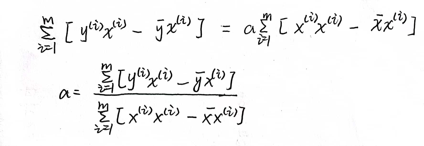
1. 简单的线性回归


2. 简单线性回归Code
导包和画图
import numpy as np
import matplotlib.pyplot as plt

x = np.array([1., 2., 3., 4., 5.])
y = np.array([1., 3., 2., 3., 5.])
plt.scatter(x, y)
plt.axis([0, 6, 0, 6])
plt.show()
拟合直线,这个是循环的方式
a_ = None
b_ = None
def fit(x_train, y_train):
        x_mean = np.mean(x_train)
        y_mean = np.mean(y_train)

        num = 0.0
        d = 0.0
        for x, y in zip(x_train, y_train):
            num += (x - x_mean) * (y - y_mean)
            d += (x - x_mean) ** 2

        a = num / d
        b = y_mean - a * x_mean

        return (a,b)

a_, b_ = fit(x,y)
y_hat = a_ * x + b_
plt.scatter(x, y)
plt.plot(x, y_hat, color='r')
plt.axis([0, 6, 0, 6])
plt.show()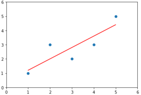
向量直接点乘的方式,效率更高:
a_ = None
b_ = None

def fit2(x_train, y_train):
        x_mean = np.mean(x_train)
        y_mean = np.mean(y_train)

        num = (x_train - x_mean).dot(y_train - y_mean)
        d = (x_train - x_mean).dot(x_train - x_mean)

        a = num / d
        b = y_mean - a * x_mean

        return (a,b)

a_, b_ = fit(x,y)
y_hat = a_ * x + b_
plt.scatter(x, y)
plt.plot(x, y_hat, color='r')
plt.axis([0, 6, 0, 6])
plt.show()
3. 多元线性回归
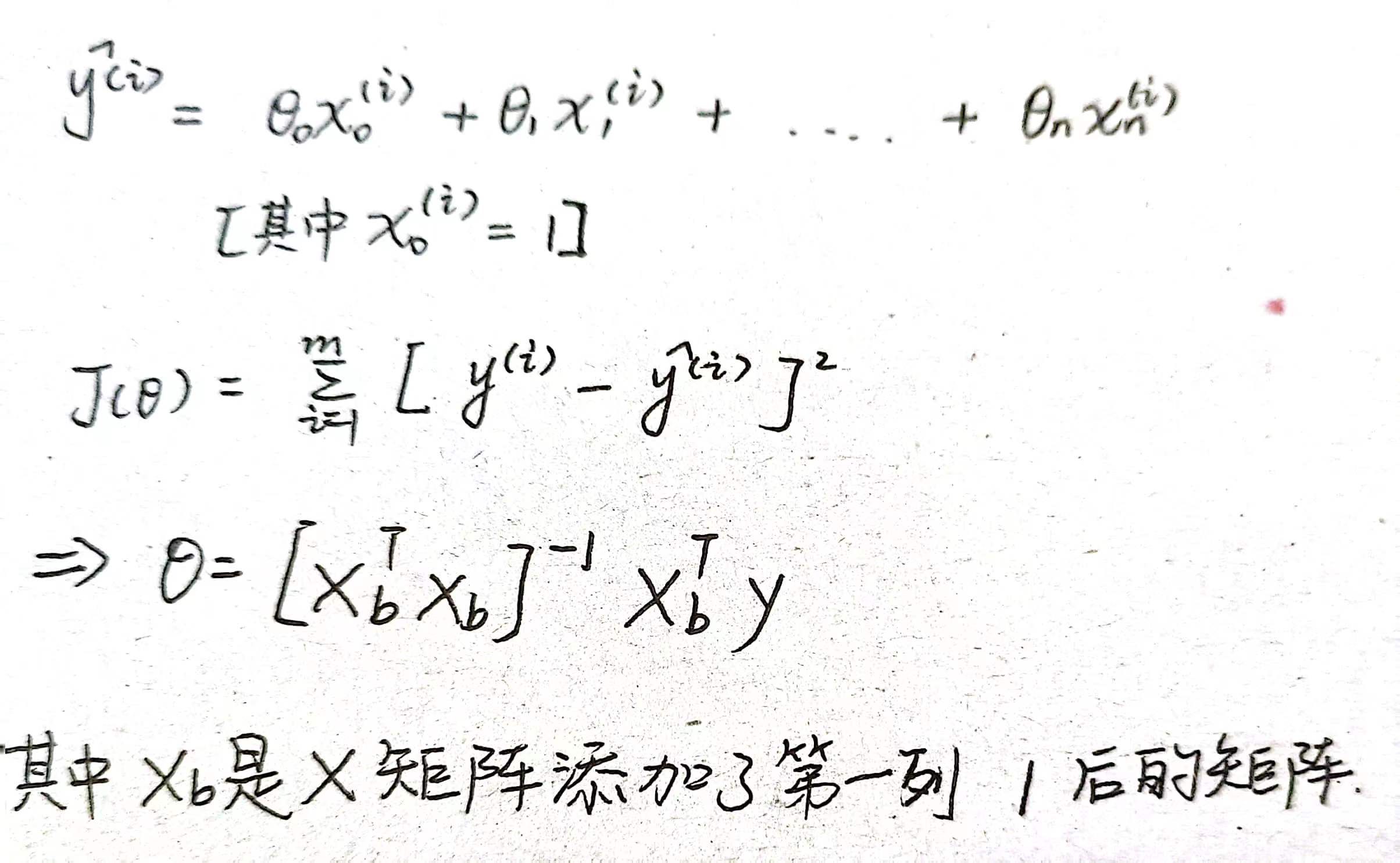
4. 多元线性回归Code
from sklearn import datasets
import numpy as np

boston = datasets.load_boston()
X = boston.data
y = boston.target
# 截距
intercept_ = None
# 其他系数
coef_ = None

def fit_normal(X_train, y_train):
    # 为 X_train 添加一列构造成 X_b
    X_b = np.hstack([np.ones((len(X_train), 1)), X_train])
    # 正规方程
    _theta = np.linalg.inv(X_b.T.dot(X_b)).dot(X_b.T).dot(y_train)

    intercept_ = _theta[0]
    coef_ = _theta[1:]

    # 以元组的形式返回 截距 和 其他系数的向量
    return (intercept_, coef_)
intercept_, coef_ = fit_normal(X, y)
print(intercept_)
print(coef_)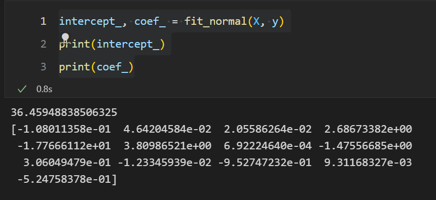
调调库,可以看到跟上面的结果是一样的。
lin_reg = LinearRegression()
lin_reg.fit(X, y)
5. 一元二次函数多元回归问题
一元二次函数:y = 0.5 * x^2 + x + 1 + 噪声
import numpy as np
import matplotlib.pyplot as plt
from sklearn.linear_model import LinearRegression

x = np.random.uniform(-3, 3, size=100)
X = x.reshape(-1, 1)
y = 0.5 * x**2 + x + 1 + np.random.normal(0, 1, 100)

plt.scatter(x, y)
plt.show()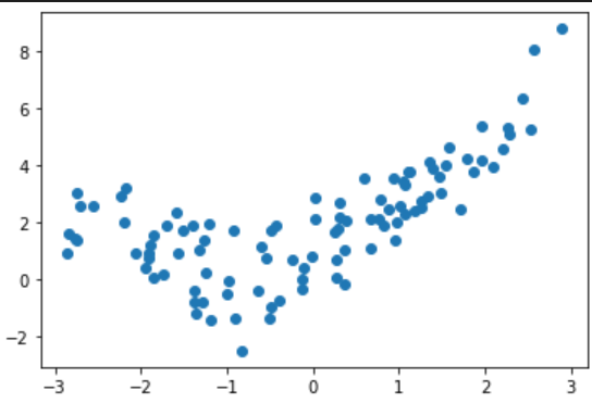
把 X^2 当成是一项
X2 = np.hstack([X, X**2])再丢到线性回归里面去
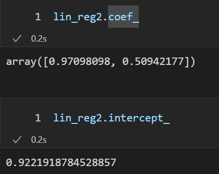
lin_reg2 = LinearRegression()
lin_reg2.fit(X2, y)
拟合出偏置项和系数
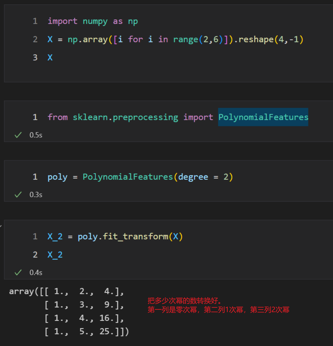
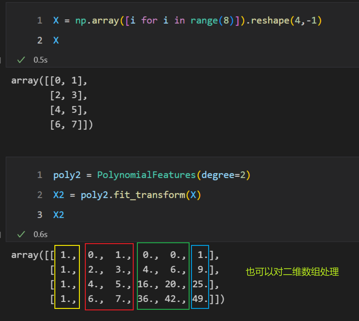
6. 多项式特征
sklearn中有一个多项式特征的工具,叫PolynomialFeatures
7. 几种误差
先给几个好解释的例子
import numpy as np
import matplotlib.pyplot as plt

x = np.random.uniform(0, 6, size=100)
X = x.reshape(-1, 1)
y = 2 * x + 1 + np.random.normal(0, 1, 100)

plt.scatter(x,y)
plt.show()
from sklearn.linear_model import LinearRegression

lin_reg = LinearRegression()
lin_reg.fit(X,y)
y_hat = lin_reg.coef_[0] * x + lin_reg.intercept_
plt.scatter(x,y)
plt.plot(np.sort(x), y_hat[np.argsort(x)], color="r")
plt.show()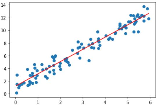
y_hat = lin_reg.predict(X)7.1 均方误差 MSE
from sklearn.metrics import mean_squared_error
MSE = mean_squared_error(y,y_hat)
MSE
7.2 均方根误差 RMSE
from math import sqrt
RMSE = sqrt(mean_squared_error(y,y_hat))
7.3 平均绝对误差 MAE
from sklearn.metrics import mean_absolute_error
MAE = mean_absolute_error(y,y_hat)
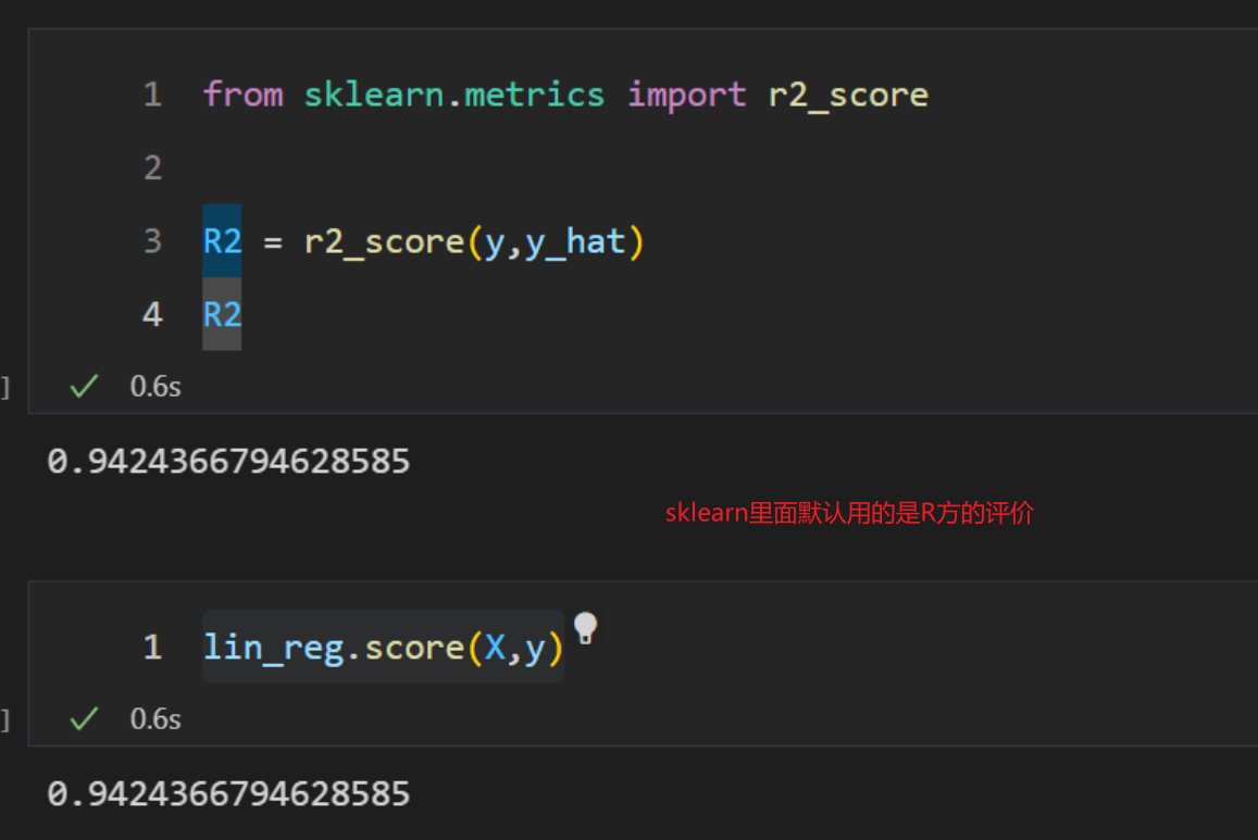
MAE7.4 R方
from sklearn.metrics import r2_score

R2 = r2_score(y,y_hat)
R2