旷视研究院CVPR2020--《Learning Relation and Topology for Occluded Person Re-Identification》

在研究行人重识别的时候意外的关注到了旷视科技，这个论文主要在于解决被遮挡的人重新识别（ReID）的目的是通过非关节摄像机将被遮挡的人图像与整体图像进行匹配。

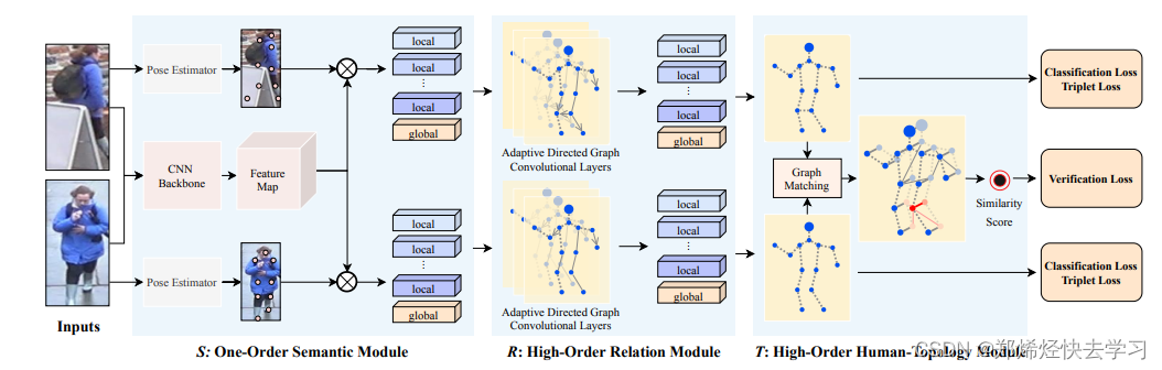
旷视科技研究团队在这篇论文中提出了一个新的框架用于解决遮挡问题，并取得了一定的效果。为了获得遮挡ReID更加鲁棒性的对齐能力，本文提出了一种新的框架，来学习具有判别力特征和人体拓扑信息的高阶关系。

论文地址：https://arxiv.org/pdf/2003.08177.pdf

GitHub：https://github.com/wangguanan/HOReID

官方：https://zhuanlan.zhihu.com/p/116014484

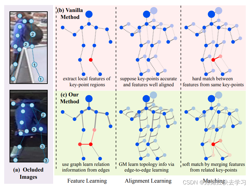
行人重识别（ReID）任务的目标是去匹配不同摄像机拍摄到的同一个人的图像，它广泛应用于视频分析、智慧城市等领域。虽然近年来提出了很多针对ReID的方法，然而，它们大多侧重于人的全身图像，忽略了更具有挑战性且也是实际应用中经常出现的行人遮挡问题。

这篇论文所运用的数据集也几乎都是有遮挡现象的数据，这种数据如果使用了前面所说的类似于切割取特征的做法可能无法做好最好，切割后只能运用到一小部分：

那么旷视如何去改进这个问题：

• 数据重构：Occluded-DukeMTMC(query里全是遮蔽现象的数据)
• 提出了三阶段模型：
  1. 关键点局部特征提取（关节点的联系，协同运动，身体组等进行分类判断）
  2. 图卷积融合关键点特征（综合利用关节点的信息，使用拓扑结构）
  3. 基于图匹配的方式来计算相似度并训练模型（遮挡做相似度计算）

总结起来就是分三阶段来完成特征提取，重点要解决遮蔽现象的局部特征。

0x01 关键点局部特征提取

• 选择一个pose estimation模型即可，得到的是各个关键点的热度图信息，通过热度图得到原始特征图的局部特征。

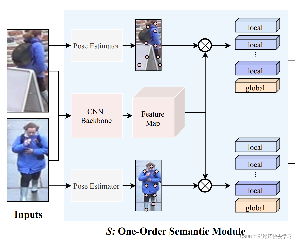
首先拿一共pose，输出每个关节点的坐标，当作是个回归任务，之后通过resnet50得到一些基本的特征，再与关节图相乘，其实就是把某个关节点的信息，强调出来。最后得到了13个local的关节点信息，以及一个全局global的信息，以上就可以得到关键点的热度图信息了，那么如何制作热度图：

其实就是一个乘法操作，用pose estimation得到的热度图来计算局部特征，左图可以理解为CNN Backbone->Feature Map，右图就是关键点信息的热度图：

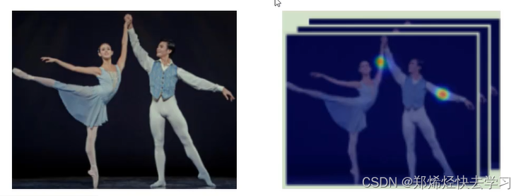
越关键的信息，颜色会越深，可以看作是权重矩阵，把权重矩阵乘上resnet50得到的特征图，即可得到当前关键点的特征图。

跟上一篇算法一样，这里同样也加了很多损失，也是局部损失以及全局损失，目的是为了再第一阶段可以更好的提特征，全局特征是通过global average pooling得到的。

总结来说：在S中，首先利用CNN backbone学习特征图，用人体关键点估计模型来学习关键点，然后，提取对应关键点的语义信息。

通过S模块后，每张输入图片都可以提取到14个特征图（13个关键点的局部特征+1个全局特征）。

0x02 局部特征关系整合（图卷积）

• 如何才能更好地利用局部特征？——加入关系。先初始化邻接矩阵来进行图卷积，邻接矩阵在学习过程中更新（如何才能更好的针对每个输入利用不同的局部特征）。
  

先说说图卷积：其实总结起来就是如何利用各个点的特征。

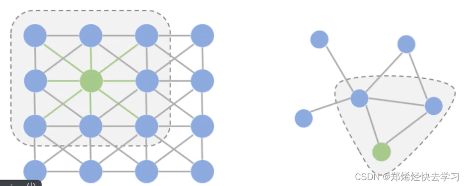
左图是我们经常使用的卷积，只要在范围内滑动就可以了。但是如果是右图的图卷积，为的是得到各个节点之间的关系，比如说头、脖子、肩膀，可以构成三角关系，脖子下面，则是各种身体部位的关系，使用这就不可以用普通卷积来做了，需要针对每个点进行零界点计算，得到当前的计算结果。

在这个任务中，就是得到邻接矩阵A来指导每个关键点特征如何跟其他关键点特征进行计算，并且A矩阵也要进行学习，要不断的更新，类似于权重参数。

这样感觉可以完美匹配人的姿态了，告诉他人长什么样子。

那么在网络中如何实现？利用差异特征来学习邻接矩阵A。

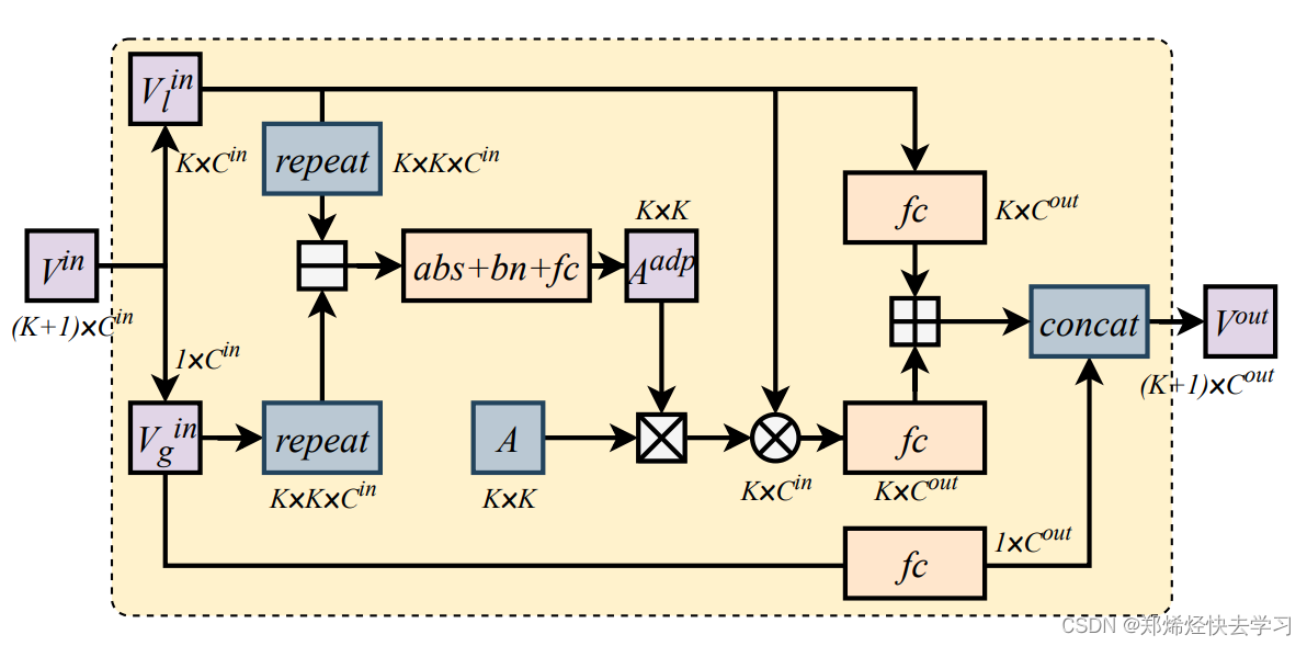
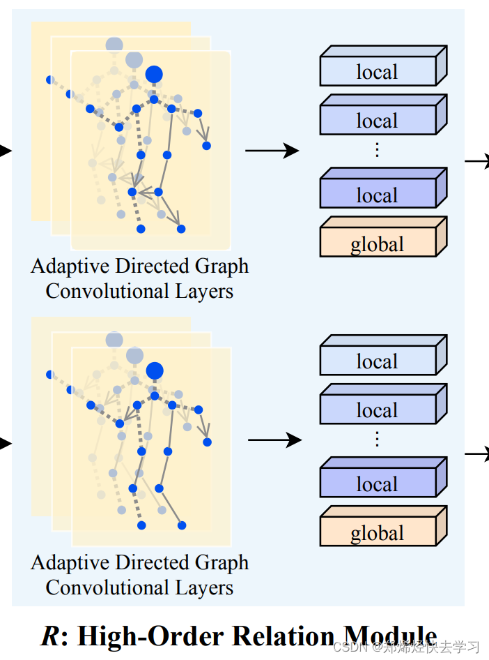
将得到的14个特征图送入文本提出的方向自适应的图卷积层（ADGC），得到新的特征信息：

• 先将局部特征VI和全局特征Vg做减法操作，得到局部特征和全局特征之间的差异特征，差异值越大，说明特征信息越不重要，属于离群信息，也就是可能被遮挡的局部特征；差异值越小，代表和全局特征越相似，该局部特征也就越重要，起的作用越大。
• 将得到的差异特征矩阵Aadp和预定义的图邻接矩阵A做点乘，得到新的邻接矩阵（表示特征点之间的relation），再和VI做矩阵乘法。
• 本身局部特征VI和关系特征融合（concat），得到带有关系的拓扑图结构信息特征。

总结来说：在R中，人们将习得的图像语义特征看作图的节点，然后提出了一个方向自适应的图卷积层（ADGC/Adaptive-Direction Graph Convolutional）层来学习和传递边缘特征信息。ADGC层可以自动决定每个边的方向和度。从而促进语义特征的信息传递，抑制无意义和噪声特征的传递。最后，学习到的节点包含语义和关系信息。

通过R模块后得到的新的13个关键点的局部特征不仅有自身的特征信息还携带了相关节点的特征信息。有了这个邻接矩阵A来进行图卷积，用它来指导如何利用不同关键点的特征进行组合，最终再与输入的局部特征进行整合。

0x03 图匹配

• 细心的人会发现在前面的训练都用的是两张图象，需要得到两个结果，其实他在后面为的就是图匹配。为什么要进行图匹配：回到了AP、AN的问题。输入两张图像（经过了前两阶段后的结果），之后计算他们之间的相似度，第一组AP，第二组AN。

• 图匹配就是要一个相似度矩阵U，例如14*14，表示两个图之间的关系，注意这里是一个交叉的过程（cross），分别交叉来得到各自匹配的特征结果。具体步骤如下：

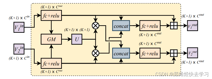
（1）对于两张图片的输入特征V1、V2，先经过全连接层(fc+relu)后进行图匹配操作（GM），得到一个关系矩阵U（代表两张图片中每个关节之间的一一对应关系）。

（2）将关系矩阵U与v1做矩阵乘法，提取V1中与V2有关系的特征，再和V2特征融合（concat），最终得到新的V2out输出特征，该特征包含V2本身特征信息和V1中与V2有关的信息。

（3）将新得到的V1out和V2out做损失优化。分别做三元组损失，还有分类损失，两个之间还需要做验证损失，其实就是sigmoid(emb1,emb2)的结果。

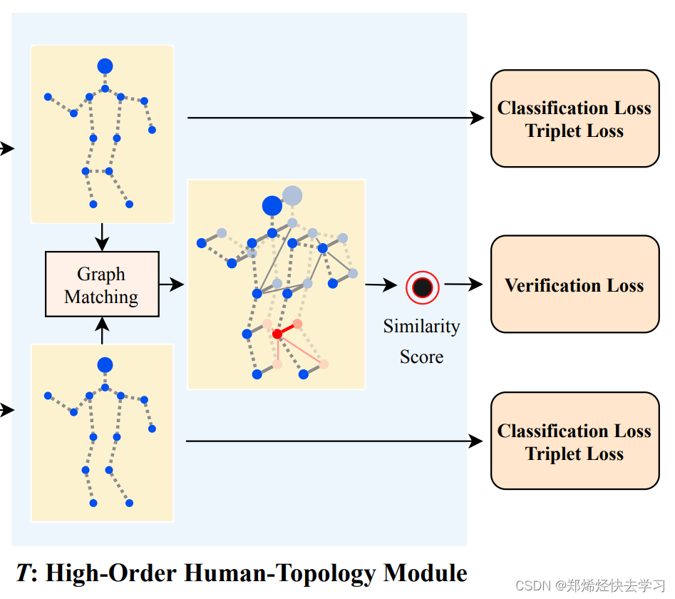
总结来说： 在T中，提出一个跨图嵌入对齐（CGEA/cross-graph embedded-alignment）层。它以两个图（graph）作为输入，利用图匹配策略学习其之间节点的对应关系，然后将学习到的对应关系视为邻接矩阵来传递信息。正因如此，相关联的特征才能被增强，对齐信息才能被嵌入到特征中去。最后，为了避免强行一对一对齐的情况，研究员会通过将两个图映射到到一个logit模型并用一个验证损失进行监督来预测其相似性。

0x04 整体算法框架分析

从上面的分析可以看出其实每个框架都是恰到好处，把图像该运用到的东西都用的淋漓尽致，可以说是一篇很值得看的论文了。

旷视研究院提出的框架，包括一个一阶语义模块（S），它可以取人体关键点区域的语义特征；一个高阶关系模块（R），它能对不同语义局部特征之间的关系信息进行建模；一个高阶人类拓扑模块（T），它可以学习到鲁棒的对齐能力，并预测两幅图像之间的相似性。这三个模块以端到端的方式进行联合训练。

0x05 数据集与环境配置

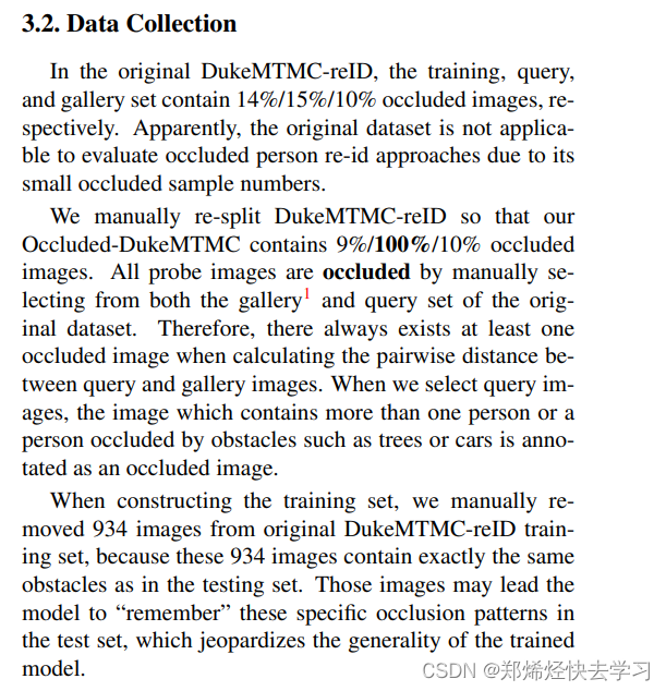
由于我们需要有遮挡现象的数据集，下面这篇论文对原始的数据集DukeMTMC -reID进行了改进：

来提取出我们需要的遮挡的数据集，可以使用下面的python代码：

import os
import shutil
import sys
from zipfile import ZipFile


target_dir = './Occluded_Duke/'
origin_duke_dir = os.path.join(target_dir,'DukeMTMC-reID') # the temp folder to save the extracted images
zip_file = './DukeMTMC-reID.zip'

def read_origin_duke_zip():
    #zip_file = sys.argv[1] # path to the origin DukeMTMC-reID.zip 
	#zip_file = './DukeMTMC-reID.zip'

    if not os.path.isfile(zip_file) or zip_file.split('/')[-1] != 'DukeMTMC-reID.zip':
        raise ValueError('Wrong zip file. Please provide correct zip file path')
    print("Extracting zip file")
    with ZipFile(zip_file) as z:
        z.extractall(path=target_dir)
        print("Extracting zip file done")


def makedir_if_not_exists(path):
    if not os.path.exists(path):
        os.makedirs(path)


def generate_new_split(split, folder_name):
    # read the re-splited name lists
    with open(os.path.join(target_dir,'{}.list'.format(split)),'r') as f:
        imgs=f.readlines()

    source_split = os.path.join(origin_duke_dir, folder_name)
    target_split = os.path.join(target_dir, folder_name)
    if not os.path.exists(target_split):
        os.makedirs(target_split)

    for img in imgs:
        img = img[:-1]
        target_path = os.path.join(target_split, img)        
        if os.path.isfile(os.path.join(source_split, img)):         
            # If the image is kept in its origin split 
            source_img_path = os.path.join(source_split, img)
        else:
            # If the image is moved to another split
            # We move some occluded images from the gallery split to the new query split
            source_img_path = os.path.join(origin_duke_dir, 'bounding_box_test', img) 
        shutil.copy(source_img_path, target_path)
    print("Generate {} split finished.".format(folder_name))


def main():
    # extract the origin DukeMTMC-reID zip, and save images to a temp folder
    read_origin_duke_zip()

    # generate the new dataset
    generate_new_split(split="train", folder_name='bounding_box_train')
    generate_new_split(split="gallery", folder_name='bounding_box_test')
    generate_new_split(split="query", folder_name='query')

    # remove the temp folder
    shutil.rmtree(origin_duke_dir)

    print("\nSuccessfully generate the new Occluded-DukeMTMC dataset.")
    print("The dataset folder is {}".format(target_dir))


if __name__ == '__main__':
    main()

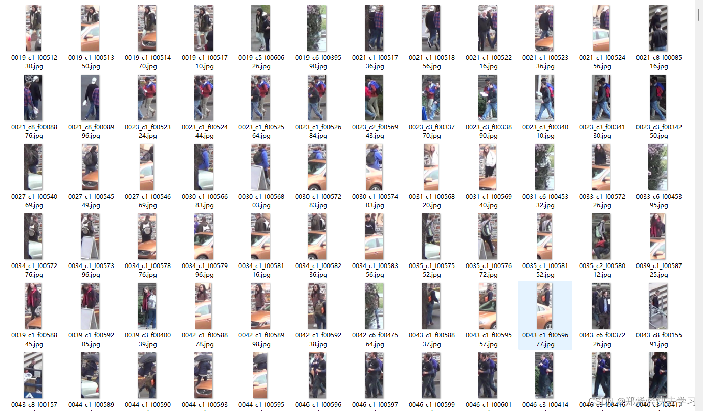
上面这段代码就可以将我们的数据集进行重构，突出我们遮挡的重点。重构的思想大家可以好好的去阅读一遍论文，最后总结是这么说的：

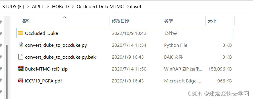
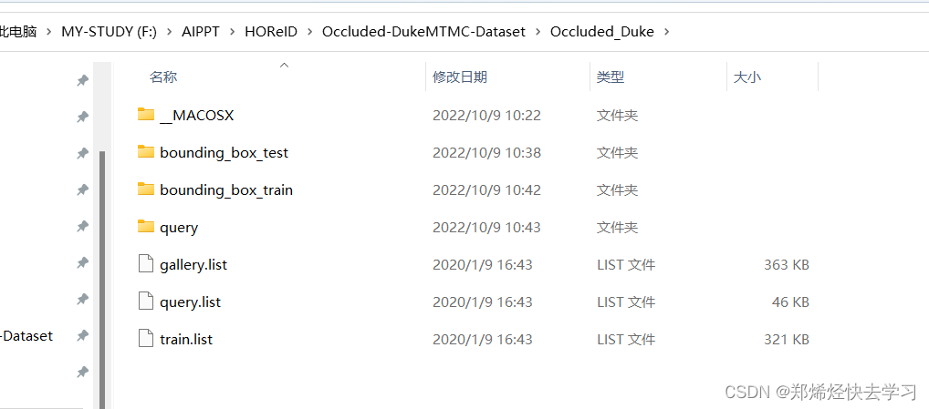
最后的数据集是这个样子的：

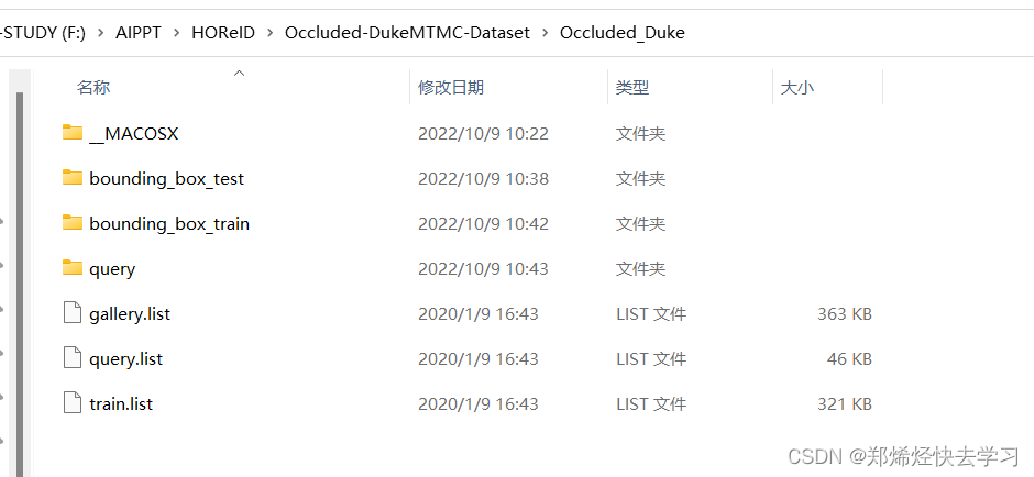
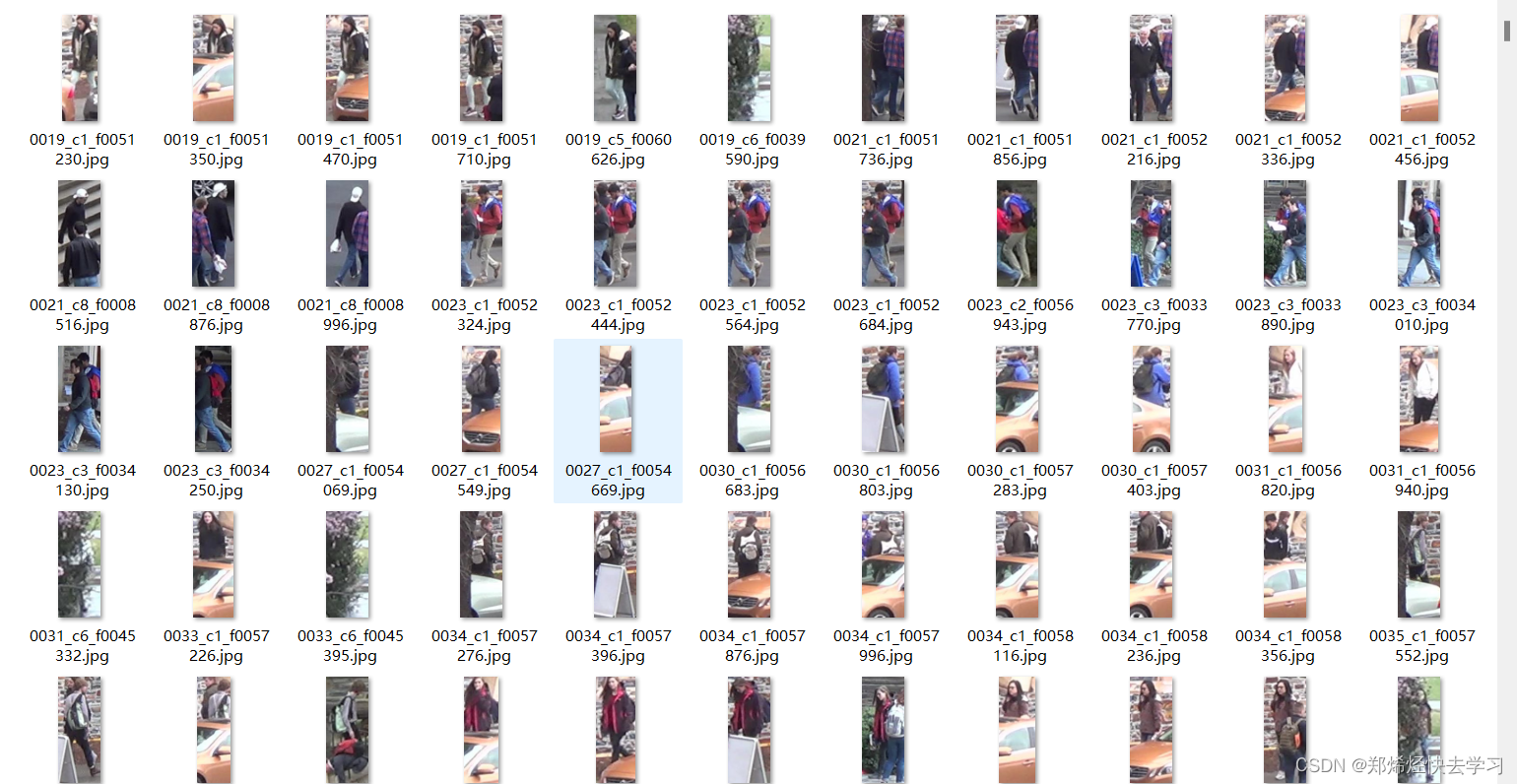
可以发现query的数据集中，几乎都是有遮挡现象的数据集：

环境配置：

conda create -n horeid python=3.7
conda activate horeid
conda install pytorch==1.1.0 torchvision==0.3.0 -c pytorch

训练时：

python 
--mode train
--duke_path ./Occluded-DukeMTMC-Dataset/Occluded_Duke
--output_path ./results

测试时：

--mode test
--resume_test_path ./pre-trainedModels 
--resume_test_epoch 119
--duke_path ./Occluded-DukeMTMC-Dataset/Occluded_Duke
--output_path ./results

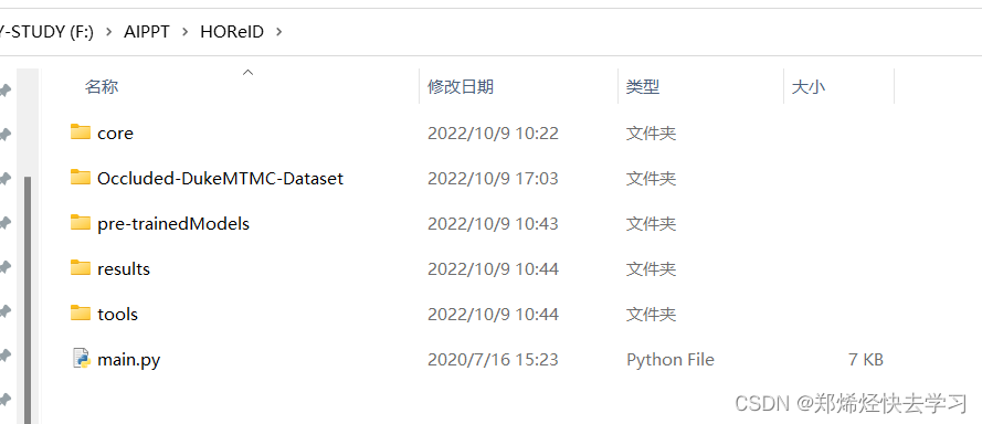
我的路径是这个样子的：

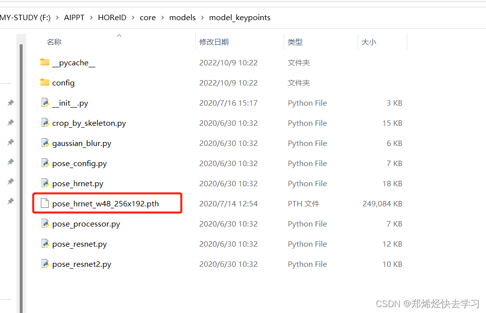
0x06 源码详解

在源码中调用了一个这个东西，可以直接识别出人体的关节点：

那么正式进入源码叭。下面这段位于base.py:

    def forward(self, images, pids, training):

        # feature
        #print(images.shape) # 16 3 256 128
        feature_maps = self.encoder(images)
        #print(feature_maps.shape)# 16 2048 16 8
        with torch.no_grad():
            score_maps, keypoints_confidence, _ = self.scoremap_computer(images)
            #print(score_maps.shape)#16 13 16 8
            #print(keypoints_confidence.shape)# 16 13
        feature_vector_list, keypoints_confidence = compute_local_features(
            self.config, feature_maps, score_maps, keypoints_confidence)

在这个地方就可以得到我们13个特征了，之后我们就需要计算局部特征的关系了。

def compute_local_features(config, feature_maps, score_maps, keypoints_confidence):
    '''
    the last one is global feature
    :param config:
    :param feature_maps:
    :param score_maps:
    :param keypoints_confidence:
    :return:
    '''
    fbs, fc, fh, fw = feature_maps.shape
    sbs, sc, sh, sw = score_maps.shape
    assert fbs == sbs and fh == sh and fw == sw

    # get feature_vector_list
    feature_vector_list = []
    for i in range(sc + 1):
        if i < sc:  # skeleton-based local feature vectors
            #这里做了个repeat操作，求出代表
            score_map_i = score_maps[:, i, :, :].unsqueeze(1).repeat([1, fc, 1, 1])#16 2048 16 8
            #print(score_map_i.shape)
            feature_vector_i = torch.sum(score_map_i * feature_maps, [2, 3])
            #print(score_map_i.shape)
            feature_vector_list.append(feature_vector_i)
        else:  # global feature vectors
            #global做一次pooling就行了
            feature_vector_i = (
                        F.adaptive_avg_pool2d(feature_maps, 1) + F.adaptive_max_pool2d(feature_maps, 1)).squeeze()
            feature_vector_list.append(feature_vector_i)
            keypoints_confidence = torch.cat([keypoints_confidence, torch.ones([fbs, 1]).cuda()], dim=1)

在上面就实现了局部特征以及整体特征了，一共14个。在这里就可以得到所有的特征啦，也就是上面那个forward调用的函数。那么回到forward，这个时候我们已经找到了14个特征了，这个时候要进行分类：

       bned_feature_vector_list, cls_score_list = self.bnclassifiers(feature_vector_list)

在model_reid.py中，我们可以看到这个处理：

    def __call__(self, feature_vector_list):

        assert len(feature_vector_list) == self.branch_num

        # bnneck for each sub_branch_feature
        bned_feature_vector_list, cls_score_list = [], []
        for i in range(self.branch_num):
            feature_vector_i = feature_vector_list[i]
            classifier_i = getattr(self, 'classifier_{}'.format(i))
            #求得分类结果
            bned_feature_vector_i, cls_score_i = classifier_i(feature_vector_i)

            bned_feature_vector_list.append(bned_feature_vector_i)
            cls_score_list.append(cls_score_i)

        return bned_feature_vector_list, cls_score_list

返回的是特征还有得分值。

下一步就是我们的图卷积了，首先先将我们的图卷积进行初始化：

 # GCN 一共形成了16个边
        self.linked_edges = \
            [[13, 0], [13, 1], [13, 2], [13, 3], [13, 4], [13, 5], [13, 6], [13, 7], [13, 8], [13, 9], [13, 10],
             [13, 11], [13, 12],  # global
             [0, 1], [0, 2],  # head
             [1, 2], [1, 7], [2, 8], [7, 8], [1, 8], [2, 7],  # body
             [1, 3], [3, 5], [2, 4], [4, 6], [7, 9], [9, 11], [8, 10], [10, 12],  # libs
             # [3,4],[5,6],[9,10],[11,12], # semmetric libs links
             ]
        self.adj = generate_adj(self.branch_num, self.linked_edges, self_connect=0.0).to(self.device)
        self.gcn = GraphConvNet(self.adj, 2048, 2048, 2048, self.config.gcn_scale).to(self.device)

在图卷积初始化的时候，先根据人的结构，先定义头身体等各个部位的关系，我们先需要存在这么一条边。之后将其描绘下来，放在一个14*14的矩阵中，这个矩阵需要训练的，当每个数据进来后要进行更新学习，这个矩阵只会改变我们初始化的那些地方，其他地方会被限制，只能利用我们拓扑图中的边。

 # gcn
        gcned_feature_vector_list = self.gcn(feature_vector_list)
        bned_gcned_feature_vector_list, gcned_cls_score_list = self.bnclassifiers2(gcned_feature_vector_list)

在这就是进行图卷积的地方。输入的是14个特征。

def generate_adj(node_num, linked_edges, self_connect=1):
    '''
    Params:
        node_num: node number
        linked_edges: [[from_where, to_where], ...]
        self_connect: float,
    '''

    if self_connect > 0:
        adj = np.eye(node_num) * self_connect
    else:
        adj = np.zeros([node_num] * 2)

    for i, j in linked_edges:
        adj[i, j] = 1.0
        adj[j, i] = 1.0

    # we suppose the last one is global feature
    adj[-1, :-1] = 0
    adj[-1, -1] = 1
    print(adj)

    adj = torch.from_numpy(adj.astype(np.float32))
    return adj

这个地方就是初始化我们的矩阵了，有边的初始化为1，没边的初始化为0。下面这个类顾名思义就是我们的第二阶段的处理了。

接下来是要进行图卷积了：

    def __call__(self, feature_list):
        cated_features = [feature.unsqueeze(1) for feature in feature_list]
        cated_features = torch.cat(cated_features, dim=1)# 16 14 2048
        #print(cated_features.shape)
        middle_features = self.adgcn1(cated_features)
        out_features = self.adgcn2(middle_features)

        out_feats_list = []
        for i in range(out_features.shape[1]):
            out_feat_i = out_features[:, i].squeeze(1)
            out_feats_list.append(out_feat_i)

        return out_feats_list

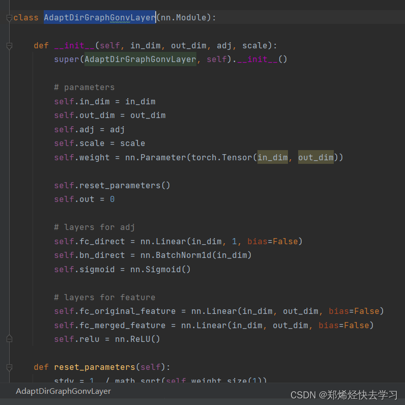
首先是把我们的特征传进去，进行拼接，拼接后就进行邻接矩阵的学习：

    def forward(self, inputs):

        # learn adj
        adj2 = self.learn_adj(inputs, self.adj)
        #print(inputs.shape)#16 14 2048
        #print(adj2.shape)
        # merge feature
        merged_inputs = torch.matmul(adj2, inputs)# b 14 2048
        #print(merged_inputs.shape)
        outputs1 = self.fc_merged_feature(merged_inputs)
        #print(outputs1.shape)
        # embed original feature
        outputs2 = self.fc_original_feature(inputs)
        #print(outputs2.shape)

        outputs = self.relu(outputs1) + outputs2
        #print(outputs.shape)
        return outputs

在这里可以算出差异特征，之后去判断这个点是否接近全局，基于差异再重新组合邻接矩阵。这一句self.learn_adj(inputs, self.adj)就是把我们的特征点，与邻接矩阵传进去求解。

    def learn_adj(self, inputs, adj):

        # inputs [bs, k(node_num), c]
        bs, k, c = inputs.shape

        #复制操作，方便减法
        global_features = inputs[:, k - 1, :].unsqueeze(1).repeat([1, k, 1])  # [bs,k,2048]
        distances = torch.abs(inputs - global_features)  # [bs, k, 2048],全局特征与各关键点之间的差异

        # bottom triangle
        distances_gap = []
        position_list = []
        for i, j in itertools.product(list(range(k)), list(range(k))):#14 * 14
            if i < j and (i != k - 1 and j != k - 1) and adj[i, j] > 0:
                #关节点之间的关系，14跟14之间的关系
                distances_gap.append(distances[:, i, :].unsqueeze(1) - distances[:, j, :].unsqueeze(1))
                position_list.append([i, j])
        distances_gap = 15 * torch.cat(distances_gap, dim=1)  # [bs, edge_number, 2048]
        #print(distances_gap.shape)
        #更新邻接矩阵，特征进行转换为输出值，现在矩阵的值已经不会只是0和1了
        adj_tmp = self.sigmoid(self.scale * self.fc_direct(
            self.bn_direct(distances_gap.transpose(1, 2)).transpose(1, 2))).squeeze()  # [bs, edge_number]
        #print(adj_tmp.shape)#16 16 之前定义好的16个边

        # re-assign
        # 学习完后重新赋值
        adj2 = torch.ones([bs, k, k]).cuda()
        for indx, (i, j) in enumerate(position_list):
            adj2[:, i, j] = adj_tmp[:, indx] * 2
            adj2[:, j, i] = (1 - adj_tmp[:, indx]) * 2
        #print(adj2.shape)# 16 14 14
        # 构建mask，只会更新我们有边的位置，其他位置继续为0
        mask = adj.unsqueeze(0).repeat([bs, 1, 1])
        #print(mask.shape)#16 14 14
        new_adj = adj2 * mask
        #print(new_adj.shape)
        #归一化
        new_adj = F.normalize(new_adj, p=1, dim=2)
		
        return new_adj

这样就可以更新邻接矩阵，并且可以得到各个关节的关系了。那么再次回到forward，把我们的邻接矩阵作用到我们的关节点信息上：

 merged_inputs = torch.matmul(adj2, inputs)# b 14 2048

之后再来一层fc：

outputs1 = self.fc_merged_feature(merged_inputs)

再与原始特征做一个整合，继续fc：

		#原始
    	outputs2 = self.fc_original_feature(inputs)
        #print(outputs2.shape)
		#两个特征加起来
        outputs = self.relu(outputs1) + outputs2
        #print(outputs.shape)
        return outputs

最后再输出为一个list：

    def __call__(self, feature_list):
        cated_features = [feature.unsqueeze(1) for feature in feature_list]
        cated_features = torch.cat(cated_features, dim=1)# 16 14 2048
        #print(cated_features.shape)
        middle_features = self.adgcn1(cated_features)
        out_features = self.adgcn2(middle_features)

        out_feats_list = []
        for i in range(out_features.shape[1]):
            out_feat_i = out_features[:, i].squeeze(1)
            out_feats_list.append(out_feat_i)

        return out_feats_list

输出后做一共分类损失以及三元组损失：

bned_gcned_feature_vector_list, gcned_cls_score_list = self.bnclassifiers2(gcned_feature_vector_list)

在以上就可以完成S与R的操作，其实跟attention是挺像的，接下来是图匹配的过程。

那么接下来就需要在训练的时候输入AP与AN了：

if training:

    # mining hard samples
    new_bned_gcned_feature_vector_list, bned_gcned_feature_vector_list_p, bned_gcned_feature_vector_list_n = mining_hard_pairs(
        bned_gcned_feature_vector_list, pids)

输入特征以及pid编号，传进去后做一个余弦相似度的矩阵，做一个16*16的矩阵，做一个label矩阵，取现在是哪个人，之后进行计算距离，进行排序，之后取一个最近的，然后再取一个最远的：

def mining_hard_pairs(feature_vector_list, pids):

    global_feature_vectors = feature_vector_list[-1]
    dist_matrix = cosine_dist(global_feature_vectors, global_feature_vectors)#16 16
    label_matrix = label2similarity(pids, pids).float()# 16 16

    _, sorted_mat_distance_index = torch.sort(dist_matrix + (9999999.) * (1 - label_matrix), dim=1, descending=False)
    hard_p_index = sorted_mat_distance_index[:, 0]
    _, sorted_mat_distance_index = torch.sort(dist_matrix + (-9999999.) * (label_matrix), dim=1, descending=True)
    hard_n_index = sorted_mat_distance_index[:, 0]

    new_feature_vector_list = []
    p_feature_vector_list = []
    n_feature_vector_list = []
    for feature_vector in feature_vector_list:
        print(feature_vector.shape)#16 2048
        feature_vector = copy.copy(feature_vector)
        new_feature_vector_list.append(feature_vector.detach())
        feature_vector = copy.copy(feature_vector.detach())
        p_feature_vector_list.append(feature_vector[hard_p_index, :])
        print(feature_vector[hard_p_index, :].shape)#16 2048
        feature_vector = copy.copy(feature_vector.detach())
        n_feature_vector_list.append(feature_vector[hard_n_index, :])
        print(feature_vector[hard_n_index, :].shape)

    return new_feature_vector_list, p_feature_vector_list, n_feature_vector_list

那么得到AN\AP后，就要走网络模型了：

# graph matching
#AP
s_p, emb_p, emb_pp = self.gmnet(new_bned_gcned_feature_vector_list, bned_gcned_feature_vector_list_p, None)
#AN
s_n, emb_n, emb_nn = self.gmnet(new_bned_gcned_feature_vector_list, bned_gcned_feature_vector_list_n, None)

接下来就是图匹配了，对两张图的14个点进行图匹配，相互之间的关系，最后可以得到14*14的相似度矩阵U，之后要分别作用在两张图上，之后把自身的特征提取到彼此身上，最后再加上fc+relu，就可以得到两个向量了，然后进行sigmoid来得到AP和AN的结果。

    def forward(self, emb1_list, emb2_list, adj):

        if type(emb1_list).__name__ == type(emb2_list).__name__ == 'list':
            emb1 = torch.cat([emb1.unsqueeze(1) for emb1 in emb1_list], dim=1)# b 14 2048
            emb2 = torch.cat([emb2.unsqueeze(1) for emb2 in emb2_list], dim=1)
        else:
            emb1 = emb1_list
            emb2 = emb2_list
        #print(emb1.shape)
        #print(emb2.shape)
        org_emb1 = emb1
        org_emb2 = emb2

        ns_src = (torch.ones([emb1.shape[0]]) * 14).int()#16
        ns_tgt = (torch.ones([emb2.shape[0]]) * 14).int()#16
        #print(ns_src.shape)
        #print(ns_tgt.shape)
		#计算相似度矩阵
        for i in range(self.GNN_LAYER):
            gnn_layer = getattr(self, 'gnn_layer_{}'.format(i))
            emb1, emb2 = gnn_layer([adj, emb1], [adj, emb2])
            #print(emb1.shape) # 16 14 1024
            affinity = getattr(self, 'affinity_{}'.format(i))
            s = affinity(emb1, emb2)
            #print(s.shape)# 16 14 14
            s = self.voting_layer(s, ns_src, ns_tgt)
            #print(s.shape)# 16 14 14
            s = self.bi_stochastic(s, ns_src, ns_tgt)
            #print(s.shape)# 16 14 14
			#这里就是交叉融合
            if i == self.GNN_LAYER - 2:
                emb1_before_cross, emb2_before_cross = emb1, emb2
                #print(emb1_before_cross.shape)
                cross_graph = getattr(self, 'cross_graph_{}'.format(i))
                emb1 = cross_graph(torch.cat((emb1_before_cross, torch.bmm(s, emb2_before_cross)), dim=-1))
                #print(emb1.shape)
                emb2 = cross_graph(torch.cat((emb2_before_cross, torch.bmm(s.transpose(1, 2), emb1_before_cross)), dim=-1))
                #print(emb2.shape)
        fin_emb1 = org_emb1 + torch.bmm(s, org_emb2)
        #print(fin_emb1.shape)
        fin_emb2 = org_emb2 + torch.bmm(s.transpose(1,2), org_emb1)
        #print(fin_emb1.shape)

        return s, fin_emb1, fin_emb2
   

结束后则要进行计算损失：

ver_prob_p = self.verificator(emb_p, emb_pp)
ver_prob_n = self.verificator(emb_n, emb_nn)

计算损失使用的是这个类：

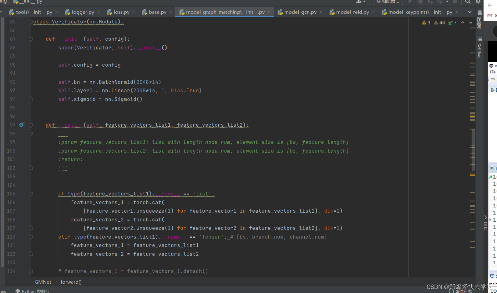
主要损失代码：

 def __call__(self, feature_vectors_list1, feature_vectors_list2):
        '''
        :param feature_vectors_list1: list with length node_num, element size is [bs, feature_length]
        :param feature_vectors_list2: list with length node_num, element size is [bs, feature_length]
        :return:
        '''


        if type(feature_vectors_list1).__name__ == 'list':
            feature_vectors_1 = torch.cat(
                [feature_vector1.unsqueeze(1) for feature_vector1 in feature_vectors_list1], dim=1)
            feature_vectors_2 = torch.cat(
                [feature_vector2.unsqueeze(1) for feature_vector2 in feature_vectors_list2], dim=1)
        elif type(feature_vectors_list1).__name__ == 'Tensor': # [bs, branch_num, channel_num]
            feature_vectors_1 = feature_vectors_list1
            feature_vectors_2 = feature_vectors_list2

        # feature_vectors_1 = feature_vectors_1.detach()
        # feature_vectors_2 = feature_vectors_2.detach()

        feature_vectors_1 = F.normalize(feature_vectors_1, p=2, dim=2)
        feature_vectors_2 = F.normalize(feature_vectors_2, p=2, dim=2)

        features = self.config.ver_in_scale * feature_vectors_1 * feature_vectors_2
        features = features.view([features.shape[0], features.shape[1] * features.shape[2]])

        logit = self.layer1(features)
        prob = self.sigmoid(logit)

        return prob

在这里就结束了三个阶段了，最后使用sigmoid后的值去判断现在是不是一个人，在这边就结束了前向传播。

0x07 跑模型时遇到的问题

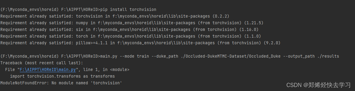
使用了我上面的命令安装东西后，准备运行的时候报错了：

(F:\Myconda_envs\horeid) F:\AIPPT\HOReID>main.py --mode train --duke_path ./Occluded-DukeMTMC-Dataset/Occluded_Duke --output_path ./results
Traceback (most recent call last):
  File "F:\AIPPT\HOReID\main.py", line 1, in <module>
    import torchvision.transforms as transforms
ModuleNotFoundError: No module named 'torchvision'

之后我尝试执行：

conda install torchvision -c pytorch

但是也没办法解决这个问题。我就试着：

pip install torchvision

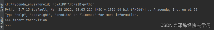
还是没有办法解决这个问题。那我们就导入模块看看是什么问题叭：

(F:\Myconda_envs\horeid) F:\AIPPT\HOReID>python
Python 3.7.13 (default, Mar 28 2022, 08:03:21) [MSC v.1916 64 bit (AMD64)] :: Anaconda, Inc. on win32
Type "help", "copyright", "credits" or "license" for more information.
>>> import torchvision
Traceback (most recent call last):
  File "<stdin>", line 1, in <module>
  File "F:\Myconda_envs\horeid\lib\site-packages\torchvision\__init__.py", line 2, in <module>
    from torchvision import datasets
  File "F:\Myconda_envs\horeid\lib\site-packages\torchvision\datasets\__init__.py", line 9, in <module>
    from .fakedata import FakeData
  File "F:\Myconda_envs\horeid\lib\site-packages\torchvision\datasets\fakedata.py", line 3, in <module>
    from .. import transforms
  File "F:\Myconda_envs\horeid\lib\site-packages\torchvision\transforms\__init__.py", line 1, in <module>
    from .transforms import *
  File "F:\Myconda_envs\horeid\lib\site-packages\torchvision\transforms\transforms.py", line 17, in <module>
    from . import functional as F
  File "F:\Myconda_envs\horeid\lib\site-packages\torchvision\transforms\functional.py", line 5, in <module>
    from PIL import Image, ImageOps, ImageEnhance, PILLOW_VERSION
ImportError: cannot import name 'PILLOW_VERSION' from 'PIL' (F:\Myconda_envs\horeid\lib\site-packages\PIL\__init__.py)
>>>

网上查到说是Pillow版本（9.2）与我们的torchvision不匹配：

pip uninstall Pillow

这个时候我们尝试将pillow安装为更低的版本：

pip install Pillow==6.1

成功解决：

新的报错：

(F:\Myconda_envs\horeid) F:\AIPPT\HOReID>python main.py --mode train --duke_path ./Occluded-DukeMTMC-Dataset/Occluded_Duke --output_path ./results
Traceback (most recent call last):
  File "main.py", line 7, in <module>
    from core import Loaders, Base, train_an_epoch, testwithVer2, visualize_ranked_images
  File "F:\AIPPT\HOReID\core\__init__.py", line 1, in <module>
    from .data_loader import Loaders
  File "F:\AIPPT\HOReID\core\data_loader\__init__.py", line 9, in <module>
    from tools import *
  File "F:\AIPPT\HOReID\tools\__init__.py", line 3, in <module>
    from .evaluation import *
  File "F:\AIPPT\HOReID\tools\evaluation\__init__.py", line 2, in <module>
    from .retrieval2 import *
  File "F:\AIPPT\HOReID\tools\evaluation\retrieval2.py", line 2, in <module>
    from sklearn import metrics as sk_metrics
ModuleNotFoundError: No module named 'sklearn'

再安装这么几个包：

pip install sklearn
pip install yacs

这个模型就可以跑了，但是在跑的过程中有这个错：

Traceback (most recent call last):
  File "main.py", line 164, in <module>
    main(config)
  File "main.py", line 69, in main
    _, results = train_an_epoch(config, base, loaders, current_epoch)
  File "F:\AIPPT\HOReID\core\train.py", line 45, in train_an_epoch
    acc = base.compute_accuracy(cls_score_list, pids)
  File "F:\AIPPT\HOReID\core\base.py", line 118, in compute_accuracy
    acc = accuracy(overall_cls_score, pids, [1])[0]
  File "F:\AIPPT\HOReID\tools\evaluation\classification.py", line 8, in accuracy
    correct = pred.eq(target.view(1, -1).expand_as(pred))
RuntimeError: Expected object of scalar type Long but got scalar type Int for argument #2 'other'

尝试着在后面加个.long()操作：

 correct = pred.eq(target.view(1, -1).expand_as(pred).long())

即可解决。