多元分类和神经网络
代码分析
首先导入需要的类库
import numpy as np
import matplotlib.pyplot as plt
import pandas as pd
import scipy.io #Used to load the OCTAVE *.mat files
import scipy.misc #Used to show matrix as an image
import matplotlib.cm as cm #Used to display images in a specific colormap
import random #To pick random images to display
from scipy.special import expit #Vectorized sigmoid function
from scipy import optimize
#可选
%matplotlib inline
1.Multi-class Classification
导入数据
#导入.mat数据
datafile = 'data/ex3data1.mat'
mat = scipy.io.loadmat( datafile )
X, y = mat['X'], mat['y']
#在X矩阵前插入全为1的一列
X = np.insert(X,0,1,axis=1)
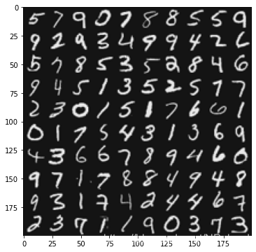
#X有5000张图片,每张图片大小20x20,共有400+1=401个像素点
#y有5000个值,值的集合为0-9
测试
print ("'y' shape: %s. Unique elements in y: %s"%(y.shape,np.unique(y)))
print ("'X' shape: %s. X[0] shape: %s"%(X.shape,X[0].shape))
输出
'y' shape: (5000, 1). Unique elements in y: [ 1  2  3  4  5  6  7  8  9 10]
'X' shape: (5000, 401). X[0] shape: (401,)
将400的行向量转为20x20的ndarray的函数
def getDatumImg(row):
    width, height = 20, 20
    #row.shape=401
    #将400的行向量转为20x20的narray
    square = row[1:].reshape(width,height)
    return square.T
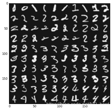
可视化数据为黑白图片
def displayData(X,indices_to_display = None):
    #图片格式为20x20
    width, height = 20, 20
    #10x10的图像网格
    nrows, ncols = 10, 10
    #5000张图片中随机抽取100张
    if not indices_to_display:
        indices_to_display = random.sample(range(X.shape[0]), nrows*ncols)
    #200x200的narray
    big_picture = np.zeros((height*nrows,width*ncols))
    #遍历图片集,为空白的大图片赋值
    irow, icol = 0, 0
    for idx in indices_to_display:
        if icol == ncols:
            irow += 1
            icol  = 0
        iimg = getDatumImg(X[idx])
        #将这块区域的图片赋值
        big_picture[irow*height:irow*height+iimg.shape[0],icol*width:icol*width+iimg.shape[1]] = iimg
        icol += 1
    #输出图片
    fig = plt.figure(figsize=(6,6))
    plt.imshow(big_picture,cmap ='gray')
测试
displayData(X)
下面我们将使用logistic regression算法来进行多元分类
如果使用向量化代替for-loop来遍历样本集,模型的训练速度会提升

下面开始将logistic regression算法向量化
首先,这是带有正则化参数的logistic regression的代价函数
J ( θ ) = − 1 m [ ∑ i = 1 m y ( i ) l o g h θ ( x ( i ) ) + ( 1 − y ( i ) ) l o g ( 1 − h θ ( x ( i ) ) ) ] + λ 2 m ∑ j = 1 n θ j 2 J(\theta)=-\frac{1}{m}[\sum_{i=1}^{m}y^{(i)}logh_{\theta}(x^{(i)})+(1-y^{(i)})log(1-h_{\theta}(x^{(i)}))]+\frac{\lambda}{2m}\sum_{j=1}^{n}\theta_{j}^{2} J(θ)=−m1[i=1∑my(i)loghθ(x(i))+(1−y(i))log(1−hθ(x(i)))]+2mλj=1∑nθj2
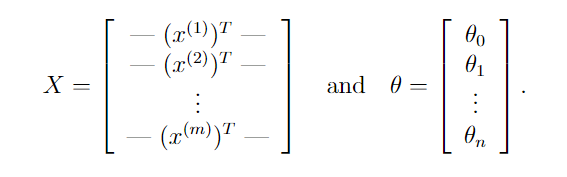
我们将X设为样本集,θ为列向量,每个元素为某一层的参数

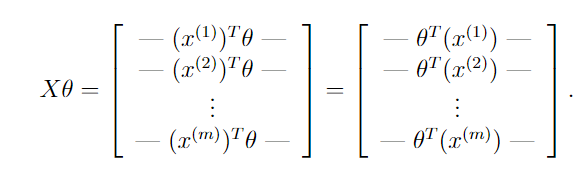
下图开始推导 θ T x ( i ) \theta^{T}x^{(i)} θTx(i)
下图开始推导 ∂ J ∂ θ j \frac{\partial J}{\partial\theta_{j}} ∂θj∂J
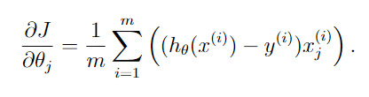
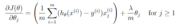
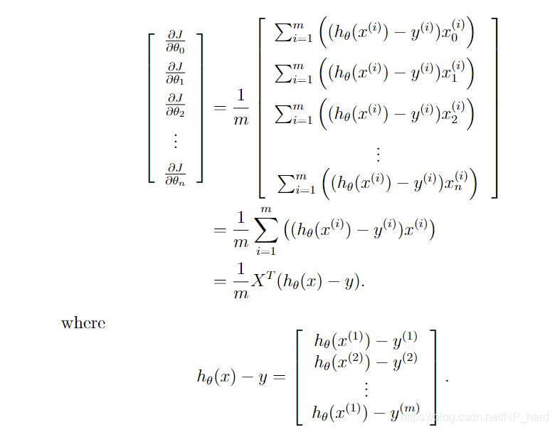

算法向量化完毕
这是hypothesis函数
def h(mytheta,myX): #Logistic hypothesis function
    return expit(np.dot(myX,mytheta))
这是计算代价的函数
def computeCost(mytheta,myX,myy,mylambda = 0.):#带有正则化参数的代价函数
    m = myX.shape[0] #5000
    myh = h(mytheta,myX) #假设值,shape: (5000,1)
    term1 = np.log( myh ).dot( myy.T ) #shape: (5000,5000)
    term2 = np.log( 1.0 - myh ).dot( 1 - myy.T ) #shape: (5000,5000)
    #原项
    left_hand = -(term1 + term2) / m #shape: (5000,5000)
    #正则项
    right_hand = mytheta.T.dot( mytheta ) * mylambda / (2*m) #shape: (1,1)
    return left_hand + right_hand #shape: (5000,5000)
开始进行多元分类
梯度计算(计算J对θ的导数)函数
#梯度计算,即计算J对θ的导数
def costGradient(mytheta,myX,myy,mylambda = 0.):
    m = myX.shape[0]
    #β=h(x)-y
    beta = h(mytheta,myX)-myy.T #shape: (5000,5000)
    #正则化项
    regterm = mytheta[1:]*(mylambda/m) #shape: (400,1)
    #J对θ的导数
    grad = (1./m)*np.dot(myX.T,beta) #shape: (401, 5000)
    grad[1:] = grad[1:] + regterm
    return grad #shape: (401, 5000)
最优化函数,返回最优θ
#最优化算法,寻找θ值
def optimizeTheta(mytheta,myX,myy,mylambda=0.):
    result = optimize.fmin_cg(computeCost, fprime=costGradient, x0=mytheta, \
                              args=(myX, myy, mylambda), maxiter=50, disp=False,\
                              full_output=True)
    return result[0], result[1]
该函数为每个输出优化一个参数列表theta
#为每个输出优化一个参数列表theta
def buildTheta(X,y):
    mylambda = 0.
    initial_theta = np.zeros((X.shape[1],1)).reshape(-1)
    Theta = np.zeros((10,X.shape[1]))
    for i in range(10):
        iclass = i if i else 10 #class 10对应0
        print ("Optimizing for handwritten number %d..."%i)
        logic_Y = np.array([1 if x == iclass else 0 for x in y])#.reshape((X.shape[0],1))
        #最优化
        itheta, imincost = optimizeTheta(initial_theta,X,logic_Y,mylambda)
        #将Theta的第i行赋值为优化后的参数
        Theta[i,:] = itheta
    print ("Done!")
    return Theta
测试
Theta = buildTheta(X,y)
print(Theta.shape)
输出
Optimizing for handwritten number 0...
Optimizing for handwritten number 1...
Optimizing for handwritten number 2...
Optimizing for handwritten number 3...
Optimizing for handwritten number 4...
Optimizing for handwritten number 5...
Optimizing for handwritten number 6...
Optimizing for handwritten number 7...
Optimizing for handwritten number 8...
Optimizing for handwritten number 9...
Done!
(10, 401)
这个函数返回最有可能的那个数字
def predictOneVsAll(myTheta,myrow):
    classes = [10] + list(range(1,10))#[10, 1, 2, 3, 4, 5, 6, 7, 8, 9]
    hypots  = [0]*len(classes)#[0, 0, 0, 0, 0, 0, 0, 0, 0, 0]
    for i in range(len(classes)):
        hypots[i] = h(myTheta[i],myrow)
    #返回最可能的那个数字
    return classes[np.argmax(np.array(hypots))]
下面计算模型在训练集上的准确率
n_correct, n_total = 0., 0.
incorrect_indices = []
for irow in range(X.shape[0]):
    n_total += 1
    if predictOneVsAll(Theta,X[irow]) == y[irow]:
        n_correct += 1
    else: incorrect_indices.append(irow)
print ("Training set accuracy: %0.1f%%"%(100*(n_correct/n_total)))
Training set accuracy: 95.4%
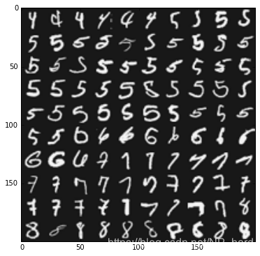
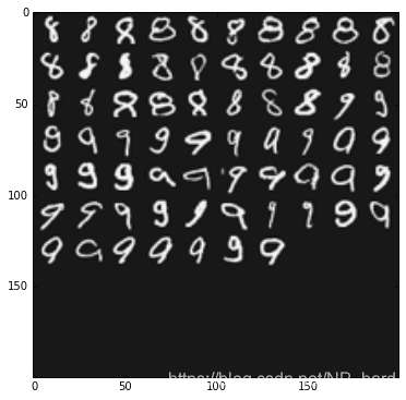
看看哪些图像识别不成功
displayData(incorrect_indices[:100])
displayData(incorrect_indices[100:200])
displayData(incorrect_indices[200:300])
神经网络
导入数据
#导入数据
datafile = 'data/ex3weights.mat'
mat = scipy.io.loadmat( datafile )
Theta1, Theta2 = mat['Theta1'], mat['Theta2']
print ("Theta1 has shape:",Theta1.shape)
print ("Theta2 has shape:",Theta2.shape)
该神经网络为双层神经网络
Theta1 has shape: (25, 401)
Theta2 has shape: (10, 26)
正向传播
#正向传播
def propagateForward(row,Thetas):
    features = row
    #循环两层
    for i in range(len(Thetas)):
        Theta = Thetas[i]
        z = Theta.dot(features) #z=θX
        a = expit(z)
        if i == len(Thetas)-1:
            return a
        #除了最后一层外都要加上bias unit
        a = np.insert(a,0,1) #Add the bias unit
        features = a
返回预测的数字
#返回预测的数字
def predictNN(row,Thetas):
    classes = list(range(1,10)) + [10]
    output = propagateForward(row,Thetas)
    #返回可能性最大的数字
    return classes[np.argmax(np.array(output))]
测试准确率
myThetas = [ Theta1, Theta2 ]
n_correct, n_total = 0., 0.
incorrect_indices = []
for irow in range(X.shape[0]):
    n_total += 1
    if predictNN(X[irow],myThetas) == int(y[irow]):
        n_correct += 1
    else: incorrect_indices.append(irow)
print ("Training set accuracy: %0.1f%%"%(100*(n_correct/n_total)))
Training set accuracy: 97.5%
看看那些识别失败的图像
for x in range(5):
    i = random.choice(incorrect_indices)
    fig = plt.figure(figsize=(3,3))
    img=X[i][1:].reshape((20,20))
    plt.imshow(img,cmap = cm.Greys_r)
    predicted_val = predictNN(X[i],myThetas)
    predicted_val = 0 if predicted_val == 10 else predicted_val
    fig.suptitle('Predicted: %d'%predicted_val, fontsize=14, fontweight='bold')


97.5 %>95.4%
神经网络模型的准确率要高
数据集
这里偷个懒,可以上kaggle上找数据