金融评分卡项目—8.逻辑回归模型在申请评分卡中的应用

文章目录

引言

一、逻辑回归概述

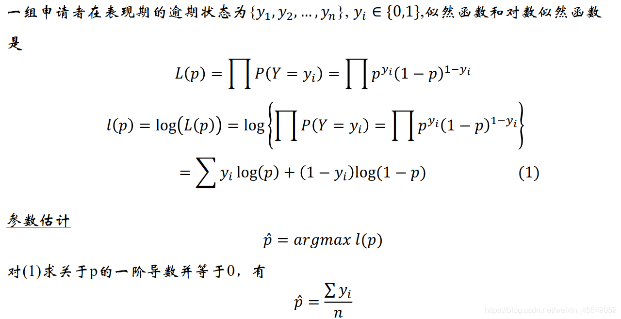
从概率的角度来看：“逾期”是一个随机事件，可以用伯努利分布来刻画它的随机性。伯努利分布是一种离散的分布，用于表示0-1型事件发生的概率。
在这里插入图片描述

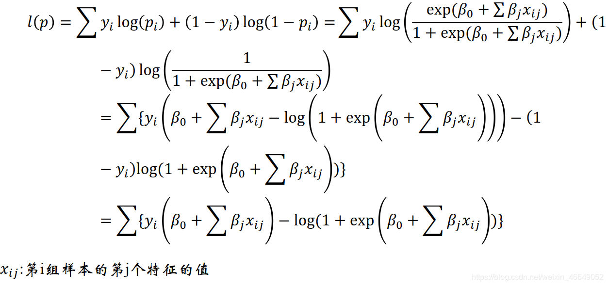
在上面的对数似然函数估计中，默认每一个样本的p是相同的，但是在申请评分卡模型中，不同申请人，逾期的概率是不同的。我们需要做的是针对不同的逾期概率区分出好样本与坏样本。

$p = f ($ x₁ $,$ x₂ $, . . .,$ x_k $)$
其中{x₁,x₂,…,x_k}是申请人的个人资质。
$p$ 是有界的，但不可直接观测。

可以用线性回归来表示 $f ()$ ?

不能，因为线性回归的 $p$ 是无界的，而在申请评分卡模型中要求 $p$ 是（0,1）。同时，也不利于通过对数似然函数来求解参数

可以用逻辑回归来表示 $f ()$ ?

可以。

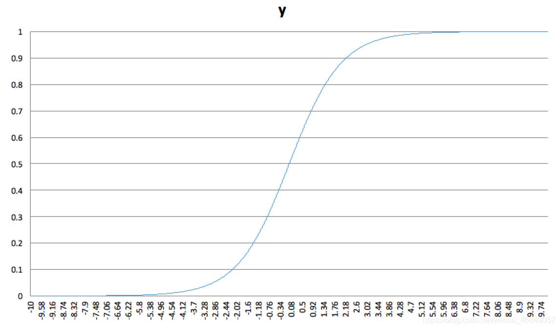
逻辑回归函数的特点：
x取值于负无穷到正无穷， $p$ 取值于(0,1)，是有界的, $f (x)$ 处处可导
其函数图像为：

对数似然函数进行参数估计：

随机梯度上升法 SGD
批量梯度上升法 min batch（常用）
针对步长，可以选用自适应步长法，根据梯度对步长进行调整

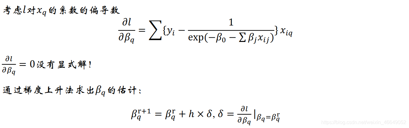
梯度上升法是逼近最大值
梯度下降法是逼近最小值

扫描二维码关注公众号，回复： 12917055 查看本文章

二、逻辑回归中的变量选择

变量挑选的作用和目的：

剔除掉跟目标变量不太相关的特征
消除多重共线性的影响
增加解释性

变量挑选与降维：
变量挑选是降维的一种手段，反之，降维并不代表着变量挑选。比如：主成分分析法（PCA）：虽然降维，但是并没有剔除变量
变量挑选的常用手段：

LASSO回归
逐步回归法
随机森林法

1.LASSO回归

LASSO全称为Least absolute sgrinkage and selection operator,对回归模型特征进行压缩估计。LASSO计算量不大，并且还可以估计出变量的重要性。
原理：
在这里插入图片描述
LASSO回归的几何解释：
详细见：L1和L2正则几何解释
假如有两个变量，其对应权重为 $w$ _$1$、 $w$ _$2$，假如| $w$ _$1$|+| $w$ _$2$|=1（l1正则化），也就是w1和w2的绝对值之和为1，则正则化等高线为正方形,红色线是损失函数的等高线
在这里插入图片描述
无论是L1正则还是L2正则，最后的最优解一定是出现在损失函数和正则等高线的焦点上。

为什么L1正则更容易导致某些W变为零，本质上是因为它在空间里面形成的等高线是尖的，在轴上它会扎到loss的等高线上，如图，β₁=0,β₂不为0，就挑选了β₂所对应的变量

超参数λ：
LASSO回归通过控制λ值来控制选择模型的特征

λ -> 0:没有正则化约束，不会剔除特征
λ ->正无穷：所有特征都不会挑选进模型
λ参数的选择非常重要，可以用交叉验证法选择最合适的λ

Group LASSO方法

可以指定一组变量同时被选进或者选出
适用于dummy encoding 和 one hot encoding

比如：针对onehot编码，只有都被选入才有意义

2.逐步回归法

逐步挑选法分为向前挑选、向后挑选与双向挑选。逐步回归法计算量大，用的不多。最常用的还是LASSO，并且LASSO还可以估计出变量的重要性。python中也没有逐步回归法的包
在这里插入图片描述

评价模型的指标有：R2，precision（精确率），AIC,BIC

AIC与BIC的区别

双向挑选用的较多，能够兼顾模型复杂度与模型精度的要求。
描述为：先两步向前挑选，再向后挑选，再反复向前向后

3.随机森林法（RF）

RF是一种集成机器学习方法，利用bootstrap和节点随机分裂技术构建多颗决策树，通过投票得到最终分类结果。RF的变量重要性度量可以作为高维数据的特征选择工具。
生成步骤：
在这里插入图片描述
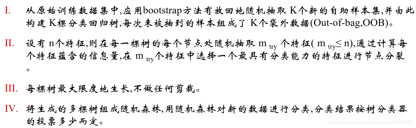
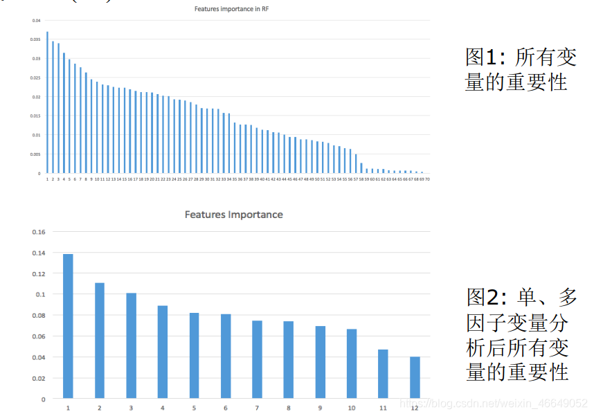
变量的重要性：
变量的重要性，即OOB数据特征发生轻微扰动后分类正确率与扰动前分类正确率的平均减少量
计算步骤为：

对于每颗决策树，利用袋外数据进行预测，将袋外数据的预测误差记录下来。其每棵树的误差是{ $e r r o r$ _$i$}
随机重排每个特征(打乱特征变量的顺序)，从而形成新的袋外数据，再利用袋外数据进行验证，其每个变量的误差是{ $e r r o r$ _$i$^`}

随机重排特征，比如：原来性别特征是男、女、男，现在变成女、女、女
对于某特征来说，计算其重要性是变换后的预测误差与原来相比的差的均值{ $e r r o r$ _$i$^` - $e r r o r$ _$i$}

将特征按重要性从高到低排列，选出前N个特征
在这里插入图片描述

GBDT模型，AdaBoost模型都有特征重要性的属性

4.挑选变量总结

LASSO法是根据超参数λ来挑选变量的，是不可控的。逐步回归法计算代价大，并且python中还没有现成的包，不建议使用。在单因子分析与多因子分析后，如果变量还多的话，可以采用随机森林法来挑选变量。

三、带权重的逻辑回归模型

在违约预测模型中，常犯两种错误：

第一类错误：将逾期人群预测成非逾期
第二类错误：将非逾期人群预测成逾期

两种误判的代价是不一样的。通过加权的方式，改善模型对于两类样本的区分。
设{ $y$ _i}对应的权重向量是{ $w$ _i},则带权重的对数似然函数是：
在这里插入图片描述
用梯度上升法求出带权重的参数估计。
评分卡模型中：

逾期样本的权重总是高于非逾期样本的权重
可以用交叉验证法选择合适的权重
也可以跟业务相结合：权重通常跟利率有关。利率高，逾期样本的权重相对低。

四、代码实现

自定义函数部分

#!usr/bin/env python
# -*- coding:utf-8 -*-
"""
@author: admin
@file: scorecardfunction.py
@time: 2021/03/12
@desc:
"""
import random
import pandas as pd
import numpy as np


def timeWindowSelection(df, daysCol, time_windows):
    """
    计算每一个时间切片内的事件的累积频率
    :param df: 数据集
    :param daysCol:时间间隔
    :param time_windows:时间窗口列表
    :return:返回覆盖度
    """
    freq_tw = {
    
    }
    for tw in time_windows:
        freq = sum(df[daysCol].apply(lambda x: int(x <= tw)))
        freq_tw[tw] = freq / df[daysCol].shape[0]
    return freq_tw


def ChangeContent(x):
    """
    数据预处理：统一大小写、统一_PHONE与_MOBILEPHONE
    :param x: UserupdateInfo1列字符
    :return:返回处理后的字符
    """
    y = x.upper()
    if y == '_MOBILEPHONE':
        y = '_PHONE'
    return y


def missingCategorical(df, x):
    """
    计算类别型变量的缺失比例
    :param df: 数据集
    :param x: 类别型变量
    :return: 返回缺失比例
    """
    missing_vals = df[x].map(lambda x: int(x != x))
    return sum(missing_vals) * 1.0 / df.shape[0]


def missingContinuous(df, x):
    """
    计算连续型变量的缺失比例
    :param df:
    :param x:
    :return:
    """
    missing_vals = df[x].map(lambda x: int(np.isnan(x)))
    return sum(missing_vals) * 1.0 / df.shape[0]


def makeUpRandom(x, sampledList):
    """
    对于连续型变量，利用随机抽样法补充缺失值
    :param x:连续型变量的值
    :param sampledList:随机抽样的列表
    :return:补缺后的值
    """
    # 非缺失，直接返回；缺失，填充后返回
    if x == x:
        return x
    else:
        return random.sample(sampledList, 1)


def AssignBin(x, cutOffPoints, special_attribute=[]):
    '''
    设置使得分箱覆盖所有训练样本外可能存在的值
    :param x: the value of variable
    :param cutOffPoints: the ChiMerge result for continous variable连续变量的卡方分箱结果
    :param special_attribute :具有特殊含义的特殊值
    :return: bin number, indexing from 0
    for example, if cutOffPoints = [10,20,30], if x = 7, return Bin 0. If x = 35, return Bin 3
    即将cutOffPoints = [10,20,30]分为4段，[0,10],(10,20],(20,30],(30,30+]
    '''
    numBin = len(cutOffPoints) + 1 + len(special_attribute)
    if x in special_attribute:
        i = special_attribute.index(x) + 1
        return 'Bin {}'.format(0 - i)
    if x <= cutOffPoints[0]:
        return 'Bin 0'
    elif x > cutOffPoints[-1]:
        return 'Bin {}'.format(numBin - 1)
    else:
        for i in range(0, numBin - 1):
            if cutOffPoints[i] < x <= cutOffPoints[i + 1]:
                return 'Bin {}'.format(i + 1)


def MaximumBinPcnt(df, col):
    """
    :param df:
    :param col:
    :return:
    """
    N = df.shape[0]
    total = df.groupby([col])[col].count()
    pcnt = total * 1.0 / N
    return max(pcnt)


def CalcWOE(df, col, target):
    '''
    计算WOE
    :param df: dataframe containing feature and target
    :param col: 需要计算WOE与IV的特征变量，通常是类别型变量
    :param target: 目标变量
    :return: WOE and IV in a dictionary
    '''
    total = df.groupby([col])[target].count()
    total = pd.DataFrame({
    
    'total': total})
    bad = df.groupby([col])[target].sum()
    bad = pd.DataFrame({
    
    'bad': bad})
    regroup = total.merge(bad, left_index=True, right_index=True, how='left')
    regroup.reset_index(level=0, inplace=True)
    # 总数量
    N = sum(regroup['total'])
    # 坏的数量
    B = sum(regroup['bad'])
    regroup['good'] = regroup['total'] - regroup['bad']
    # 好的数量
    G = N - B
    regroup['bad_pcnt'] = regroup['bad'].map(lambda x: x * 1.0 / B)
    regroup['good_pcnt'] = regroup['good'].map(lambda x: x * 1.0 / G)
    regroup['WOE'] = regroup.apply(lambda x: np.log(x.good_pcnt * 1.0 / x.bad_pcnt), axis=1)
    # 计算WOE
    WOE_dict = regroup[[col, 'WOE']].set_index(col).to_dict(orient='index')
    # 计算IV
    IV = regroup.apply(lambda x: (x.good_pcnt - x.bad_pcnt) * np.log(x.good_pcnt * 1.0 / x.bad_pcnt), axis=1)
    IV = sum(IV)
    return {
    
    "WOE": WOE_dict, 'IV': IV}


def BadRateEncoding(df, col, target):
    '''
    bad rate编码
    :param df: dataframe containing feature and target
    :param col: 需要以bad rate进行编码的特征变量，通常是类别型变量
    :param target: good/bad indicator
    :return: 返回被bad rate编码的类别型变量
    '''
    total = df.groupby([col])[target].count()
    total = pd.DataFrame({
    
    'total': total})
    bad = df.groupby([col])[target].sum()
    bad = pd.DataFrame({
    
    'bad': bad})
    regroup = total.merge(bad, left_index=True, right_index=True, how='left')
    regroup.reset_index(level=0, inplace=True)
    regroup['bad_rate'] = regroup.apply(lambda x: x.bad * 1.0 / x.total, axis=1)
    br_dict = regroup[[col, 'bad_rate']].set_index([col]).to_dict(orient='index')
    badRateEnconding = df[col].map(lambda x: br_dict[x]['bad_rate'])
    return {
    
    'encoding': badRateEnconding, 'br_rate': br_dict}


def Chi2(df, total_col, bad_col, overallRate):
    '''
    # 计算卡方值
    :param df: the dataset containing the total count and bad count
    :param total_col: total count of each value in the variable
    :param bad_col: bad count of each value in the variable
    :param overallRate: the overall bad rate of the training set—逾期率
    :return: the chi-square value
    '''
    df2 = df.copy()
    df2['expected'] = df[total_col].apply(lambda x: x * overallRate)
    combined = zip(df2['expected'], df2[bad_col])
    chi = [(i[0] - i[1]) ** 2 / i[0] for i in combined]
    chi2 = sum(chi)
    return chi2


def AssignGroup(x, bin):
    """
    将超过100个的属性值调整到100个
    :param x: 属性值
    :param bin: 99个分割点
    :return: 调整后的值
    """
    N = len(bin)
    if x <= min(bin):
        return min(bin)
    elif x > max(bin):
        return 10e10
    else:
        for i in range(N - 1):
            if bin[i] < x <= bin[i + 1]:
                return bin[i + 1]


# ChiMerge_MaxInterval:
def ChiMerge_MaxInterval_Original(df, col, target, max_interval=5):
    '''
    通过指定最大分箱数，使用卡方值拆分连续变量
    :param df: the dataframe containing splitted column, and target column with 1-0
    :param col: splitted column
    :param target: target column with 1-0
    :param max_interval: 最大分箱数
    :return: the combined bins
    '''
    colLevels = set(df[col])
    # since we always combined the neighbours of intervals, we need to sort the attributes
    # 排序
    colLevels = sorted(list(colLevels))
    N_distinct = len(colLevels)
    if N_distinct <= max_interval:
        print("The number of original levels for {} is less than or equal to max intervals".format(col))
        return colLevels[:-1]
    else:
        # Step 1: group the dataset by col and work out the total count & bad count in each level of the raw column
        # 按col对数据集进行分组，并计算出total count & bad count
        total = df.groupby([col])[target].count()
        total = pd.DataFrame({
    
    'total': total})
        bad = df.groupby([col])[target].sum()
        bad = pd.DataFrame({
    
    'bad': bad})
        regroup = total.merge(bad, left_index=True, right_index=True, how='left')
        # 重置索引，将原来的index变为数据列保留下来
        regroup.reset_index(level=0, inplace=True)
        N = sum(regroup['total'])
        B = sum(regroup['bad'])
        # the overall bad rate will be used in calculating expected bad count
        # 总的逾期率
        overallRate = B * 1.0 / N
        # 每一个属性属于一个区间
        groupIntervals = [[i] for i in colLevels]
        groupNum = len(groupIntervals)
        # 终止条件：在迭代的每个步骤中，间隔数等于预先指定的阈值（最大分箱数），我们计算每个属性的卡方值
        while (len(groupIntervals) > max_interval):
            chisqList = []
            for interval in groupIntervals:
                df2 = regroup.loc[regroup[col].isin(interval)]
                chisq = Chi2(df2, 'total', 'bad', overallRate)
                chisqList.append(chisq)
            # 找到最小卡方值的位置，并将该卡方值与左右两侧相邻的较小的卡方值合并
            min_position = chisqList.index(min(chisqList))
            if min_position == 0:
                combinedPosition = 1
            elif min_position == groupNum - 1:
                combinedPosition = min_position - 1
            else:
                if chisqList[min_position - 1] <= chisqList[min_position + 1]:
                    combinedPosition = min_position - 1
                else:
                    combinedPosition = min_position + 1
            groupIntervals[min_position] = groupIntervals[min_position] + groupIntervals[combinedPosition]
            # after combining two intervals, we need to remove one of them
            groupIntervals.remove(groupIntervals[combinedPosition])
            groupNum = len(groupIntervals)
        groupIntervals = [sorted(i) for i in groupIntervals]
        cutOffPoints = [i[-1] for i in groupIntervals[:-1]]
        return cutOffPoints


def ChiMerge_MaxInterval(df, col, target, max_interval=5, special_attribute=[]):
    '''
    通过指定最大分箱数，使用卡方值拆分连续变量
    :param df: the dataframe containing splitted column, and target column with 1-0
    :param col: splitted column
    :param target: target column with 1-0
    :param max_interval: 最大分箱数
    :return: 返回分箱点
    '''
    colLevels = sorted(list(set(df[col])))
    N_distinct = len(colLevels)
    if N_distinct <= max_interval:
        print("The number of original levels for {} is less than or equal to max intervals".format(col))
        return colLevels[:-1]
    else:
        if len(special_attribute) >= 1:
            df1 = df.loc[df[col].isin(special_attribute)]  # 是特殊属性的值
            df2 = df.loc[~df[col].isin(special_attribute)]  # 非特殊属性的值
        else:
            df2 = df.copy()
        N_distinct = len(list(set(df2[col])))
        # 如果属性过多，则时间代价较大，不妨取100个属性进行分箱
        if N_distinct > 100:
            ind_x = [int(i / 100.0 * N_distinct) for i in range(1, 100)]
            split_x = [colLevels[i] for i in ind_x]
            df2['temp'] = df2[col].map(lambda x: AssignGroup(x, split_x))
        else:
            df['temp'] = df2[col]
        # Step 1: group the dataset by col and work out the total count & bad count in each level of the raw column
        # 按col对数据集进行分组，并计算出total count & bad count
        total = df2.groupby(['temp'])[target].count()
        total = pd.DataFrame({
    
    'total': total})
        bad = df2.groupby(['temp'])[target].sum()
        bad = pd.DataFrame({
    
    'bad': bad})
        regroup = total.merge(bad, left_index=True, right_index=True, how='left')
        regroup.reset_index(level=0, inplace=True)
        N = sum(regroup['total'])
        B = sum(regroup['bad'])
        # the overall bad rate will be used in calculating expected bad count
        # 计算总的逾期率
        overallRate = B * 1.0 / N
        # initially, each single attribute forms a single interval
        # 对变量属性进行排序，因为我们要合并相邻区间
        colLevels = sorted(list(set(df2['temp'])))
        groupIntervals = [[i] for i in colLevels]
        groupNum = len(groupIntervals)
        split_intervals = max_interval - len(special_attribute)
        # 终止条件：在迭代的每个步骤中，间隔数等于预先指定的阈值（最大分箱数），我们计算每个属性的卡方值
        while (len(groupIntervals) > split_intervals):
            chisqList = []
            for interval in groupIntervals:
                df2b = regroup.loc[regroup['temp'].isin(interval)]
                chisq = Chi2(df2b, 'total', 'bad', overallRate)
                chisqList.append(chisq)
            # 找到最小卡方值的位置，并将该卡方值与左右两侧相邻的较小的卡方值合并
            min_position = chisqList.index(min(chisqList))
            if min_position == 0:
                combinedPosition = 1
            elif min_position == groupNum - 1:
                combinedPosition = min_position - 1
            else:
                if chisqList[min_position - 1] <= chisqList[min_position + 1]:
                    combinedPosition = min_position - 1
                else:
                    combinedPosition = min_position + 1
            groupIntervals[min_position] = groupIntervals[min_position] + groupIntervals[combinedPosition]
            # after combining two intervals, we need to remove one of them
            groupIntervals.remove(groupIntervals[combinedPosition])
            groupNum = len(groupIntervals)
        groupIntervals = [sorted(i) for i in groupIntervals]
        cutOffPoints = [max(i) for i in groupIntervals[:-1]]
        cutOffPoints = special_attribute + cutOffPoints
        return cutOffPoints


def BadRateMonotone(df, sortByVar, target):
    """
    分成5个箱后，判断bad rate是否是单调的，可以是单调上升，也可以是单调下降；如果不单调的话，继续合并
    :param df: DataFrame
    :param sortByVar:分箱后的变量
    :param target:目标变量
    :return: 返回是否单调
    """
    df2 = df.sort([sortByVar])
    total = df2.groupby([sortByVar])[target].count()
    total = pd.DataFrame({
    
    'total': total})
    bad = df2.groupby([sortByVar])[target].sum()
    bad = pd.DataFrame({
    
    'bad': bad})
    regroup = total.merge(bad, left_index=True, right_index=True, how='left')
    regroup.reset_index(level=0, inplace=True)
    combined = zip(regroup['total'], regroup['bad'])
    badRate = [x[1] * 1.0 / x[0] for x in combined]

    badRateMonotone = [badRate[i] < badRate[i + 1] for i in range(len(badRate) - 1)]
    Monotone = len(set(badRateMonotone))
    if Monotone == 1:
        return True
    else:
        return False


def MergeBad0(df, col, target):
    '''
    当某个或者几个类别的bad rate为0时，需要和最小的非bad rate的箱进行合并
     :param df: dataframe containing feature and target
     :param col: the feature that needs to be calculated the WOE and iv, usually categorical type
     :param target: good/bad indicator
     :return: WOE and IV in a dictionary
     '''
    total = df.groupby([col])[target].count()
    total = pd.DataFrame({
    
    'total': total})
    bad = df.groupby([col])[target].sum()
    bad = pd.DataFrame({
    
    'bad': bad})
    regroup = total.merge(bad, left_index=True, right_index=True, how='left')
    regroup.reset_index(level=0, inplace=True)
    regroup['bad_rate'] = regroup.apply(lambda x: x.bad * 1.0 / x.total, axis=1)
    # 按bad rate列进行排序
    regroup = regroup.sort_values(by='bad_rate')
    col_regroup = [[i] for i in regroup[col]]
    for i in range(regroup.shape[0]):
        col_regroup[1] = col_regroup[0] + col_regroup[1]
        col_regroup.pop(0)
        if regroup['bad_rate'][i + 1] > 0:
            break
    newGroup = {
    
    }
    for i in range(len(col_regroup)):
        for g2 in col_regroup[i]:
            newGroup[g2] = 'Bin ' + str(i)
    return newGroup


def KS_AR(df, score, target):
    '''
    计算申请评分卡模型的AR与KS值
    :param df: the dataset containing probability and bad indicator
    :param score:
    :param target:
    :return:
    '''
    total = df.groupby([score])[target].count()
    bad = df.groupby([score])[target].sum()
    all = pd.DataFrame({
    
    'total': total, 'bad': bad})
    all['good'] = all['total'] - all['bad']
    all[score] = all.index
    all = all.sort_values(by=score, ascending=False)
    all.index = range(len(all))
    all['badCumRate'] = all['bad'].cumsum() / all['bad'].sum()
    all['goodCumRate'] = all['good'].cumsum() / all['good'].sum()
    all['totalPcnt'] = all['total'] / all['total'].sum()
    arList = [0.5 * all.loc[0, 'badCumRate'] * all.loc[0, 'totalPcnt']]
    for j in range(1, len(all)):
        ar0 = 0.5 * sum(all.loc[j - 1:j, 'badCumRate']) * all.loc[j, 'totalPcnt']
        arList.append(ar0)
    arIndex = (2 * sum(arList) - 1) / (all['good'].sum() * 1.0 / all['total'].sum())

    KS = all.apply(lambda x: x.badCumRate - x.goodCumRate, axis=1)
    return {
    
    'AR': arIndex, 'KS': max(KS)}

主程序部分

#!usr/bin/env python
# -*- coding:utf-8 -*-
"""
@author: admin
@file: scorecard model feature.py
@time: 2021/03/12
@desc:
"""
import pandas as pd
import datetime
import collections
import numpy as np
import numbers
import random
import pickle
from pandas.plotting import scatter_matrix
from sklearn.linear_model import LinearRegression, LogisticRegressionCV
from itertools import combinations
from sklearn.linear_model import LinearRegression
from sklearn.ensemble import RandomForestClassifier
from sklearn.model_selection import train_test_split
import statsmodels.api as sm
from itertools import combinations
from scorecardfunction import *

# step0:读取csv文件，检查Idx的一致性
data1 = pd.read_csv('data/PPD_LogInfo_3_1_Training_Set.csv', header=0)
data2 = pd.read_csv('data/PPD_Training_Master_GBK_3_1_Training_Set.csv', header=0, encoding='gbk')
data3 = pd.read_csv('data/PPD_Userupdate_Info_3_1_Training_Set.csv', header=0)
data1_Idx, data2_Idx, data3_Idx = set(data1.Idx), set(data2.Idx), set(data3.Idx)
check_Idx_integrity = (data1_Idx - data2_Idx) | (data2_Idx - data1_Idx) | (data1_Idx - data3_Idx) | (
        data3_Idx - data1_Idx)

# step1:PPD_LogInfo_3_1_Training_Set 和 PPD_Userupdate_Info_3_1_Training_Set数据集的特征衍生
# 先对PPD_LogInfo_3_1_Training_Set数据集进行特征衍生
# 提取每一个申请人的申请时间间隔
# 登陆时间
data1['logInfo'] = data1['LogInfo3'].map(lambda x: datetime.datetime.strptime(x, '%Y-%m-%d'))
# 借款成交时间
data1['Listinginfo'] = data1['Listinginfo1'].map(lambda x: datetime.datetime.strptime(x, '%Y-%m-%d'))
# 借款成交时间-登陆时间
data1['ListingGap'] = data1[['logInfo', 'Listinginfo']].apply(lambda x: (x[1] - x[0]).days, axis=1)
# 查看不同时间切片的覆盖度，发现180天时，覆盖度达到95%
timeWindows = timeWindowSelection(data1, 'ListingGap', range(30, 361, 30))
print(timeWindows)

# 我们将时间窗口设置为[7,30,60,90,120,150,180]，在不同时间切片内衍生变量
time_window = [7, 30, 60, 90, 120, 150, 180]
# 可以衍生特征
var_list = ['LogInfo1', 'LogInfo2']
# drop_duplicates()表示去除重复项
data1GroupbyIdx = pd.DataFrame({
    
    'Idx': data1['Idx'].drop_duplicates()})
for tw in time_window:
    data1['TruncatedLogInfo'] = data1['Listinginfo'].map(lambda x: x + datetime.timedelta(-tw))  # timedelta第一个参数为day
    # 在时间间隔内的数据
    temp = data1.loc[data1['logInfo'] >= data1['TruncatedLogInfo']]
    for var in var_list:
        # count the frequences of LogInfo1 and LogInfo2——操作的次数
        count_stats = temp.groupby(['Idx'])[var].count().to_dict()
        data1GroupbyIdx[str(var) + '_' + str(tw) + '_count'] = data1GroupbyIdx['Idx'].map(
            lambda x: count_stats.get(x, 0))

        # count the distinct value of LogInfo1 and LogInfo2——不同操作类别/代码的个数
        Idx_UserupdateInfo1 = temp[['Idx', var]].drop_duplicates()
        uniq_stats = Idx_UserupdateInfo1.groupby(['Idx'])[var].count().to_dict()

        data1GroupbyIdx[str(var) + '_' + str(tw) + '_unique'] = data1GroupbyIdx['Idx'].map(
            lambda x: uniq_stats.get(x, 0))

        # calculate the average count of each value in LogInfo1 and LogInfo2—计算同一类别/代码的平均操作次数
        data1GroupbyIdx[str(var) + '_' + str(tw) + '_avg_count'] = data1GroupbyIdx[
            [str(var) + '_' + str(tw) + '_count', str(var) + '_' + str(tw) + '_unique']]. \
            apply(lambda x: x[0] * 1.0 / x[1], axis=1)

# 对PPD_Userupdate_Info_3_1_Training_Set数据集进行特征衍生
# 借款成交日期
data3['ListingInfo'] = data3['ListingInfo1'].map(lambda x: datetime.datetime.strptime(x, '%Y/%m/%d'))
# 借款人修改时间
data3['UserupdateInfo'] = data3['UserupdateInfo2'].map(lambda x: datetime.datetime.strptime(x, '%Y/%m/%d'))
# 时间间隔 = 借款成交日期 - 借款人修改时间
data3['ListingGap'] = data3[['UserupdateInfo', 'ListingInfo']].apply(lambda x: (x[1] - x[0]).days, axis=1)
# collections.Counter表示计算“可迭代序列中”各个元素（element）的数量
collections.Counter(data3['ListingGap'])
# np.histogram()是一个生成直方图的函数
# np.histogram() 默认地使用10个相同大小的区间（箱），然后返回一个元组（频数，分箱的边界）
hist_ListingGap = np.histogram(data3['ListingGap'])
hist_ListingGap = pd.DataFrame({
    
    'Freq': hist_ListingGap[0], 'gap': hist_ListingGap[1][1:]})
# 频数累加
hist_ListingGap['CumFreq'] = hist_ListingGap['Freq'].cumsum()
# 频数的百分比
hist_ListingGap['CumPercent'] = hist_ListingGap['CumFreq'].map(lambda x: x * 1.0 / hist_ListingGap.iloc[-1]['CumFreq'])
# 我们将时间窗口设置为[7,30,60,90,120,150,180]，在不同时间切片内衍生变量
# 数据预处理:统一大小写、统一Phone、Mobilephone
data3['UserupdateInfo1'] = data3['UserupdateInfo1'].map(ChangeContent)
# 去掉重复索引，添加衍生变量
data3GroupbyIdx = pd.DataFrame({
    
    'Idx': data3['Idx'].drop_duplicates()})
time_window = [7, 30, 60, 90, 120, 150, 180]

for tw in time_window:
    # 时间切片范围内的数据
    data3['TruncatedLogInfo'] = data3['ListingInfo'].map(lambda x: x + datetime.timedelta(-tw))
    temp = data3.loc[data3['UserupdateInfo'] >= data3['TruncatedLogInfo']]

    # 统计每个Idx的操作次数
    freq_stats = temp.groupby(['Idx'])['UserupdateInfo1'].count().to_dict()
    data3GroupbyIdx['UserupdateInfo_' + str(tw) + '_freq'] = data3GroupbyIdx['Idx'].map(lambda x: freq_stats.get(x, 0))

    # 统计每个Idx的操作类数
    Idx_UserupdateInfo1 = temp[['Idx', 'UserupdateInfo1']].drop_duplicates()
    # print(Idx_UserupdateInfo1)
    unique_stats = Idx_UserupdateInfo1.groupby(['Idx'])['UserupdateInfo1'].count().to_dict()
    data3GroupbyIdx['UserupdateInfo_' + str(tw) + '_unique'] = data3GroupbyIdx['Idx'].map(
        lambda x: unique_stats.get(x, x))

    # 统计每个Idx每个操作类型的平均操作次数
    data3GroupbyIdx['UserupdateInfo_' + str(tw) + '_avg_count'] = data3GroupbyIdx[
        ['UserupdateInfo_' + str(tw) + '_freq', 'UserupdateInfo_' + str(tw) + '_unique']]. \
        apply(lambda x: x[0] * 1.0 / x[1], axis=1)

    # whether the applicant changed items like IDNUMBER,HASBUYCAR, MARRIAGESTATUSID, PHONE
    # 关注特殊变量——是否修改了这些变量
    Idx_UserupdateInfo1['UserupdateInfo1'] = Idx_UserupdateInfo1['UserupdateInfo1'].map(lambda x: [x])
    # 相加
    Idx_UserupdateInfo1_V2 = Idx_UserupdateInfo1.groupby(['Idx'])['UserupdateInfo1'].sum()
    for item in ['_IDNUMBER', '_HASBUYCAR', '_MARRIAGESTATUSID', '_PHONE']:
        item_dict = Idx_UserupdateInfo1_V2.map(lambda x: int(item in x)).to_dict()
        # print(item_dict)
        data3GroupbyIdx['UserupdateInfo_' + str(tw) + str(item)] = data3GroupbyIdx['Idx'].map(
            lambda x: item_dict.get(x, x))

# 合并表格—将data2与衍生信息合并起来
allData = pd.concat([data2.set_index('Idx'), data3GroupbyIdx.set_index('Idx'), data1GroupbyIdx.set_index('Idx')],
                    axis=1)
allData.to_csv('data/allData_0.csv', encoding='gbk')

# step2:Makeup missing value for categorical variables and continuous variables
# 为类别变量与连续型变量填充缺失值

allData = pd.read_csv('data/allData_0.csv', header=0, encoding='gbk')
# allData.replace('', np.nan, inplace=True)
allFeatures = list(allData.columns)
# 移除借款成交时间与目标变量
allFeatures.remove('ListingInfo')
allFeatures.remove('target')
allFeatures.remove('Idx')

# 删除常量型特征
for col in allFeatures:
    if len(set(allData[col])) == 1:
        allFeatures.remove(col)

# 将自变量分为连续型变量与类别型变量
numerical_var = []
for var in allFeatures:
    uniq_vals = list(set(allData[var]))
    if np.nan in uniq_vals:
        uniq_vals.remove(np.nan)
    if len(uniq_vals) >= 10 and isinstance(uniq_vals[0], numbers.Real):
        numerical_var.append(var)

categorical_var = [i for i in allFeatures if i not in numerical_var]

# 删除缺失率超过50%的类别变量，剩余变量缺失作为一种状态
missing_pcnt_threshould_1 = 0.5
for var in categorical_var:
    missingRate = missingCategorical(allData, var)
    print(var, ' has missing rate as ', missingRate)
    if missingRate > missing_pcnt_threshould_1:
        categorical_var.remove(var)
        del allData[var]
    # 剩余变量将缺失当成一种状态
    if 0 < missingRate < missing_pcnt_threshould_1:
        allData[var] = allData[var].map(lambda x: "'" + str(x) + "'")

# 删除缺失率超过30%的连续型变量，剩余变量利用随机抽样法对缺失值进行补缺
missing_pcnt_threshould_2 = 0.3
for var in numerical_var:
    missingRate = missingContinuous(allData, var)
    if missingRate > missing_pcnt_threshould_2:
        numerical_var.remove(var)
        del allData[var]
        print('we delete variable {} because of its high missing rate'.format(var))
    else:
        if missingRate > 0:
            not_missing = allData.loc[allData[var] == allData[var]][var]
            # Population must be a sequence or set.  For dicts, use list(d)
            allData[var] = allData[var].map(lambda x: makeUpRandom(x, list(not_missing)))

allData.to_csv('data/allData_1.csv', header=True, encoding='gbk', columns=allData.columns, index=False)

# step3:变量分箱
# 对于每个类别变量，如果其唯一值大于5，我们将使用ChiMerge对其进行合并
trainData = pd.read_csv('data/allData_1.csv', header=0, encoding='gbk')
allFeatures = list(trainData.columns)
allFeatures.remove('ListingInfo')
allFeatures.remove('target')
allFeatures.remove('Idx')
# 数据预处理—将类别变量中大写转化成小写
for col in categorical_var:
    trainData[col] = trainData[col].map(lambda x: str(x).upper())

"""
对于类别型变量，按照下列步骤:
1.如果变量的唯一值超过5个，我们就需要分箱；计算bad rate，并以bad rate对变量进行编码，按照bad rate进行排序，计算每一对相邻区间的卡方值，
将卡方值最小的区间进行合并
2.另外,
    2.1 检查占比最高的组，如果有一组占比超过95%（90%），则删除该变量(占比高相当于常量型特征)
    2.2 检查每一个分箱的bad rate，当某个或者几个类别的bad rate为0时，需要和最小的非bad rate的箱进行合并
"""
deleted_features = []  # delete the categorical features in one of its single bin occupies more than 90%
encoded_features = []
merged_features = []
var_IV = {
    
    }  # save the IV values for binned features
var_WOE = {
    
    }
WOE_dict = {
    
    }
for col in categorical_var:
    print('we are processing {}'.format(col))
    if len(set(trainData[col])) > 5:
        print('{} is encoded with bad rate'.format(col))
        col0 = str(col) + '_encoding'
        trainData[col0] = BadRateEncoding(trainData, col, 'target')['encoding']
        # 当做连续型变量
        numerical_var.append(col0)
        encoded_features.append(col0)
        del trainData[col]
    else:
        maxPcnt = MaximumBinPcnt(trainData, col)
        if maxPcnt > 0.9:
            print('{} is deleted because of large percentage of single bin'.format(col))
            deleted_features.append(col)
            categorical_var.remove(col)
            del trainData[col]
            continue
        bad_bin = trainData.groupby([col])['target'].sum()
        if min(bad_bin) == 0:
            print('{} has 0 bad sample!'.format(col))
            # 当某个或者几个类别的bad rate为0时，需要和最小的非bad rate的箱进行合并
            mergeBin = MergeBad0(trainData, col, 'target')
            col1 = str(col) + '_mergeByBadRate'
            trainData[col1] = trainData[col].map(mergeBin)
            # 计算合并后组的最大占比
            maxPcnt = MaximumBinPcnt(trainData, col1)
            if maxPcnt > 0.9:
                print('{} is deleted because of large percentage of single bin'.format(col))
                deleted_features.append(col)
                categorical_var.remove(col)
                del trainData[col]
                continue
            WOE_IV = CalcWOE(trainData, col1, 'target')
            WOE_dict[col1] = WOE_IV['WOE']
            var_IV[col1] = WOE_IV['IV']
            merged_features.append(col)
            del trainData[col]
        else:
            WOE_IV = CalcWOE(trainData, col, 'target')
            WOE_dict[col] = WOE_IV['WOE']
            var_IV[col] = WOE_IV['IV']

"""
对于连续型变量，我们需要做如下工作：
1.按ChiMerge拆分变量（默认分为5个bin）
2.检查bate rate，如果不是单调的话，我们减少箱数，直到bate rate是单调
3.如果最大bin占用超过90％，则删除变量
"""
var_cutoff = {
    
    }
for col in numerical_var:
    print("{} is in processing".format(col))
    col1 = str(col) + '_Bin'
    # (1), split the continuous variable and save the cutoffpoints. Particulary, -1 is a special case and we separate it into a group
    if -1 in set(trainData[col]):
        special_attribute = [-1]
    else:
        special_attribute = []
    # 卡方分箱，返回分箱点
    cutOffPoints = ChiMerge_MaxInterval(trainData, col, 'target', special_attribute=special_attribute)
    var_cutoff[col] = cutOffPoints
    # 设置使得分箱覆盖所有训练样本外可能存在的值
    trainData[col1] = trainData[col].map(lambda x: AssignBin(x, cutOffPoints, special_attribute=special_attribute))

    # (2) 判断bad rate是否是单调的
    BRM = BadRateMonotone(trainData, col1, 'target', special_attribute=special_attribute)
    # 如果不单调就减少最大分箱数，进行重新分箱，再判断，直至bins=2或者bad rate单调
    if not BRM:
        for bins in range(4, 1, -1):
            cutOffPoints = ChiMerge_MaxInterval(trainData, col, 'target', max_interval=bins,
                                                special_attribute=special_attribute)
            trainData[col1] = trainData[col].map(
                lambda x: AssignBin(x, cutOffPoints, special_attribute=special_attribute))
            BRM = BadRateMonotone(trainData, col1, 'target', special_attribute=special_attribute)
            if BRM:
                break
        var_cutoff[col] = cutOffPoints

    # (3) 检查占比最高的组是否超过90%
    maxPcnt = MaximumBinPcnt(trainData, col1)
    if maxPcnt > 0.9:
        # del trainData[col1]
        deleted_features.append(col)
        numerical_var.remove(col)
        print('we delete {} because the maximum bin occupies more than 90%'.format(col))
        continue
    WOE_IV = CalcWOE(trainData, col1, 'target')
    var_IV[col] = WOE_IV['IV']
    var_WOE[col] = WOE_IV['WOE']
    del trainData[col]

trainData.to_csv('data/allData_2.csv', header=True, encoding='gbk', columns=trainData.columns, index=False)

filewrite = open('data/var_WOE.pkl', 'w')
pickle.dump(var_WOE, filewrite)
filewrite.close()

filewrite = open('data/var_IV.pkl', 'w')
pickle.dump(var_IV, filewrite)
filewrite.close()

# step4:选择IV大于0.02的变量，并进行WOE编码
trainData = pd.read_csv('data/allData_2.csv', header=0, encoding='gbk')
# 变量值转化成字符串
num2str = ['SocialNetwork_13', 'SocialNetwork_12', 'UserInfo_6', 'UserInfo_5', 'UserInfo_10', 'UserInfo_17',
           'city_match']
for col in num2str:
    trainData[col] = trainData[col].map(lambda x: str(x))

# (i) WOE编码
for col in var_WOE.keys():
    print(col)
    col2 = str(col) + "_WOE"
    # 数值型变量和部分转换成数值型变量的类别型变量
    if col in var_cutoff.keys():
        cutOffPoints = var_cutoff[col]
        special_attribute = []
        if - 1 in cutOffPoints:
            special_attribute = [-1]

        binValue = trainData[col].map(lambda x: AssignBin(x, cutOffPoints, special_attribute=special_attribute))
        # WOE编码
        trainData[col2] = binValue.map(lambda x: var_WOE[col][x])
    # 类别数小于5的类别型变量
    else:
        trainData[col2] = trainData[col].map(lambda x: var_WOE[col][x])

trainData.to_csv('data/allData_3.csv', header=True, encoding='gbk', columns=trainData.columns, index=False)

# (ii) 选择IV大于0.02的变量
iv_threshould = 0.02
varByIV = [k for k, v in var_IV.items() if v > iv_threshould]

# (iii) 检查成对woe特征的共线性
var_IV_selected = {
    
    k: var_IV[k] for k in varByIV}
var_IV_sorted = sorted(var_IV_selected.iteritems(), key=lambda d: d[1], reverse=True)
# 按IV值排序后的变量
var_IV_sorted = [i[0] for i in var_IV_sorted]

removed_var = []
roh_thresould = 0.6
for i in range(len(var_IV_sorted) - 1):
    if var_IV_sorted[i] not in removed_var:
        x1 = var_IV_sorted[i] + "_WOE"
        for j in range(i + 1, len(var_IV_sorted)):
            if var_IV_sorted[j] not in removed_var:
                x2 = var_IV_sorted[j] + "_WOE"
                # 返回皮尔逊相关系数
                roh = np.corrcoef([trainData[x1], trainData[x2]])[0, 1]
                if abs(roh) >= roh_thresould:
                    print('the correlation coeffient between {0} and {1} is {2}'.format(x1, x2, str(roh)))
                    if var_IV[var_IV_sorted[i]] > var_IV[var_IV_sorted[j]]:
                        removed_var.append(var_IV_sorted[j])
                    else:
                        removed_var.append(var_IV_sorted[i])
# 删除部分变量
var_IV_sortet_2 = [i for i in var_IV_sorted if i not in removed_var]

# (iiii) 检查多重共线性 according to VIF > 10
for i in range(len(var_IV_sortet_2)):
    x0 = trainData[var_IV_sortet_2[i] + '_WOE']
    x0 = np.array(x0)
    # 除研究变量外的其他解释变量
    X_Col = [k + '_WOE' for k in var_IV_sortet_2 if k != var_IV_sortet_2[i]]
    X = trainData[X_Col]
    X = np.matrix(X)
    regr = LinearRegression()
    clr = regr.fit(X, x0)
    x_pred = clr.predict(X)
    # R2
    R2 = 1 - ((x_pred - x0) ** 2).sum() / ((x0 - x0.mean()) ** 2).sum()
    vif = 1 / (1 - R2)
    if vif > 10:
        print("Warning: the vif for {0} is {1}".format(var_IV_sortet_2[i], vif))

# step5:在单因子分析与多因子分析后，建立逻辑回归模型
# 1.x,y
var_WOE_list = [i + '_WOE' for i in var_IV_sortet_2]
y = trainData['target']
X = trainData[var_WOE_list]
# 人为构造一个不相关的特征
X['intercept'] = [1] * X.shape[0]

# 2.利用pvalue(显著性)来挑选变量,p越小越好，越小就有更大概率拒绝原假设
LR = sm.Logit(y, X).fit()
summary = LR.summary()
pvals = LR.pvalues
pvals = pvals.to_dict()

# Some features are not significant, so we need to delete feature one by one.
varLargeP = {
    
    k: v for k, v in pvals.items() if v >= 0.1}
# 降序
varLargeP = sorted(varLargeP.items(), key=lambda d: d[1], reverse=True)
while (len(varLargeP) > 0 and len(var_WOE_list) > 0):
    # In each iteration, we remove the most insignificant feature and build the regression again, until
    # (1) all the features are significant or
    # (2) no feature to be selected
    varMaxP = varLargeP[0][0]
    if varMaxP == 'intercept':
        print('the intercept is not significant!')
        break
    var_WOE_list.remove(varMaxP)
    y = trainData['target']
    X = trainData[var_WOE_list]
    X['intercept'] = [1] * X.shape[0]

    LR = sm.Logit(y, X).fit()
    summary = LR.summary()
    pvals = LR.pvalues
    pvals = pvals.to_dict()
    varLargeP = {
    
    k: v for k, v in pvals.items() if v >= 0.1}
    varLargeP = sorted(varLargeP.items(), key=lambda d: d[1], reverse=True)

print(var_WOE_list)
'''
Now all the features are significant and the sign of coefficients are negative
var_WOE_list = ['UserInfo_15_encoding_WOE', u'ThirdParty_Info_Period6_10_WOE', u'ThirdParty_Info_Period5_2_WOE', 'UserInfo_16_encoding_WOE', 'WeblogInfo_20_encoding_WOE',
            'UserInfo_7_encoding_WOE', u'UserInfo_17_WOE', u'ThirdParty_Info_Period3_10_WOE', u'ThirdParty_Info_Period1_10_WOE', 'WeblogInfo_2_encoding_WOE',
            'UserInfo_1_encoding_WOE']
'''
# 保存模型
# 固化python变量
saveModel = open('data/LR_Model_Normal.pkl', 'w')
# 保存成二进制文件
pickle.dump(LR, saveModel)
saveModel.close()

# step6:建立带有权重的逻辑回归模型—使用LASSO进行变量挑选—指标是KS
# use cross validation to select the best regularization parameter
X = trainData[var_WOE_list]
X = np.matrix(X)
y = trainData['target']
y = np.array(y)
# 分割数据集
X_train, X_test, y_train, y_test = train_test_split(X, y, test_size=0.4, random_state=0)

model_parameter = {
    
    }
for C_penalty in np.arange(0.005, 0.2, 0.005):
    for bad_weight in range(2, 101, 2):
        LR_model_2 = LogisticRegressionCV(Cs=[C_penalty], penalty='l1', solver='liblinear', class_weight={
    
    1: bad_weight, 0: 1})
        LR_model_2_fit = LR_model_2.fit(X_train, y_train)
        y_pred = LR_model_2_fit.predict_proba(X_test)[:, 1]
        scorecard_result = pd.DataFrame({
    
    'prob': y_pred, 'target': y_test})
        performance = KS_AR(scorecard_result, 'prob', 'target')
        KS = performance['KS']
        # KS越大，模型区分能力越好
        model_parameter[(C_penalty, bad_weight)] = KS


# Step 7: build the logistic regression using according to RF feature importance

# build random forest model to estimate the importance of each feature
# In this case we use the original feautures with WOE encoding before single analysis

X = trainData[var_WOE_list]
X = np.matrix(X)
y = trainData['target']
y = np.array(y)

RFC = RandomForestClassifier()
RFC_Model = RFC.fit(X, y)
features_rfc = trainData[var_WOE_list].columns
featureImportance = {
    
    features_rfc[i]: RFC_Model.feature_importances_[i] for i in range(len(features_rfc))}
featureImportanceSorted = sorted(featureImportance.items(), key=lambda x: x[1], reverse=True)
# we selecte the top 10 features
features_selection = [k[0] for k in featureImportanceSorted[:10]]

y = trainData['target']
X = trainData[features_selection]
X['intercept'] = [1] * X.shape[0]

LR = sm.Logit(y, X).fit()
summary = LR.summary()
"""
                           Logit Regression Results
==============================================================================
Dep. Variable:                 target   No. Observations:                30000
Model:                          Logit   Df Residuals:                    29989
Method:                           MLE   Df Model:                           10
Date:                Wed, 26 Apr 2017   Pseudo R-squ.:                 0.05762
Time:                        19:26:13   Log-Likelihood:                -7407.3
converged:                       True   LL-Null:                       -7860.2
                                        LLR p-value:                3.620e-188
==================================================================================================
                                     coef    std err          z      P>|z|      [0.025      0.975]
--------------------------------------------------------------------------------------------------
UserInfo_1_encoding_WOE           -1.0433      0.135     -7.756      0.000      -1.307      -0.780
WeblogInfo_20_encoding_WOE        -0.9011      0.089    -10.100      0.000      -1.076      -0.726
UserInfo_15_encoding_WOE          -0.9184      0.069    -13.215      0.000      -1.055      -0.782
UserInfo_7_encoding_WOE           -0.9891      0.096    -10.299      0.000      -1.177      -0.801
UserInfo_16_encoding_WOE          -0.9492      0.099     -9.603      0.000      -1.143      -0.756
ThirdParty_Info_Period1_10_WOE    -0.5942      0.143     -4.169      0.000      -0.874      -0.315
ThirdParty_Info_Period2_10_WOE    -0.0650      0.165     -0.395      0.693      -0.388       0.257
ThirdParty_Info_Period3_10_WOE    -0.2052      0.136     -1.511      0.131      -0.471       0.061
ThirdParty_Info_Period6_10_WOE    -0.6902      0.090     -7.682      0.000      -0.866      -0.514
ThirdParty_Info_Period5_10_WOE    -0.4018      0.100     -4.017      0.000      -0.598      -0.206
intercept                         -2.5382      0.024   -107.939      0.000      -2.584      -2.492
==================================================================================================
"""