金融评分卡项目—4.GBDT模型在流失预警模型中的应用

文章目录

一、GBDT模型介绍

梯度提升树是一个集成模型，可用于分类、回归与排序。GBDT的核心在于累加所有树的结果作为最终结果，GBDT可用于分类，并不代表是累加所有分类树的结果。GBDT中的树都是回归树（利用平方误差最小化准则，进行特征选择，生成二叉树），不是分类树，这点对理解GBDT相当重要
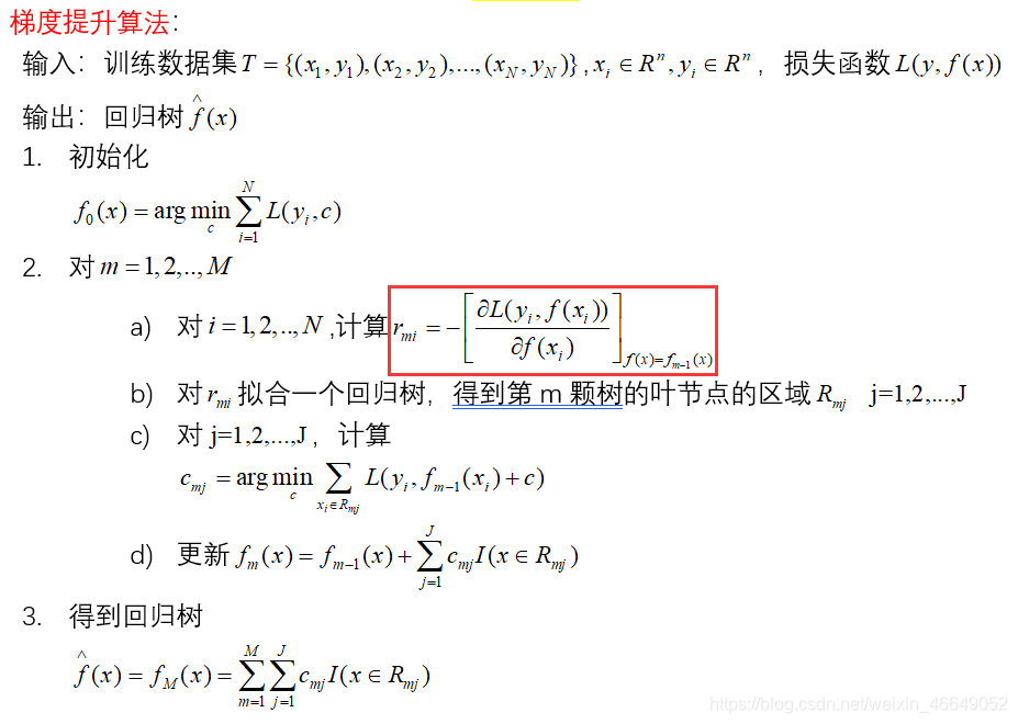
梯度提升树，当损失函数是平方损失时，下一棵树拟合的是上一棵树的残差值（实际值减预测值）。当损失函数是非平方损失时，拟合的是损失函数的负梯度值。

举个简单例子：
A的真实年龄是18岁，但第一棵树的预测年龄是12岁，差了6岁，即残差为6岁。那么在第二棵树里我们把A的年龄设为6岁去学习，如果第二棵树真的能把A分到6岁的叶子节点，那累加两棵树的结论就是A的真实年龄；如果第二棵树的结论是5岁，则A仍然存在1岁的残差，第三棵树里A的年龄就变成1岁，继续学。

当损失函数是平方差损失时，用残差作为全局最优的绝对方向，并不需要Gradient求解。但是损失函数多种多样，当损失函数是非平方损失时，机器学习界的大牛Freidman提出了梯度提升算法：利用最速下降的近似方法，即利用损失函数的负梯度在当前模型的值，作为回归问题中提升树算法的残差的近似值，拟合一个回归树。
在这里插入图片描述

特点：

基于简单回归决策树的组合模型

决策树的优点：

解释性强
允许变量交互作用
对离群值、缺失值、共线性不敏感

决策树的缺点：

准确度不够高
易过拟合
运算量大

扫描二维码关注公众号，回复： 12708103 查看本文章
沿着梯度下降的方向进行提升
只接受数值型连续变量—需要做特征转化（将类别型变量转换成离散型变量）

优点：

准确度高
不易过拟合

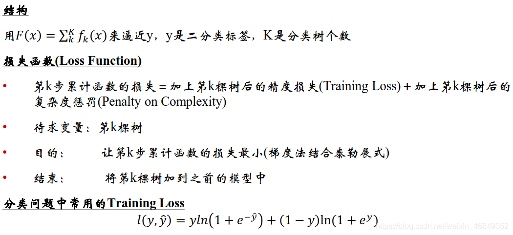
1.该案例GBDT结构

在这里插入图片描述

2.GBDT常用参数

更多参数解析详见sklearn官网
GBDT框架常用参数

n_estimators:分类树的个数，K

learning_rate:即每个弱学习器的权重缩减系数 $v$ ,也称为步长。较小的 $v$ 意味着需要更多的弱学习器的迭代次数。
参数n_estimators和learning_rate要一起调参。可以从一个小一点的 $v$ 开始调参，默认为1，这两个参数关系相反，一个大了，另一个就小了

Subsample:（不放回）抽样率，推荐[0.5,0.8]之间，默认是1.0，即不使用子采样

init:即初始化的时候的弱学习器，一般用在对数据有先验知识，或者之前做过一些拟合的时候

loss:GBDT算法中的损失函数

max_features : {‘auto’, ‘sqrt’, ‘log2’}, int or float, default=None
寻找最佳分割时需要考虑的特性数量:
If int, then consider max_features features at each split.
If float, then max_features is a fraction and int(max_features * n_features) features are considered at each split.
If ‘auto’, then max_features=sqrt(n_features).
If ‘sqrt’, then max_features=sqrt(n_features).
If ‘log2’, then max_features=log2(n_features).
If None, then max_features=n_features.

弱分类树的参数：

max_features:划分时考虑的最大特征数

max_depth:决策树的最大深度

min_samples_split:内部节点再划分时所需的最小样本数。默认是2。如果样本量不大，就不需要管这个值。如果样本量数量级非常大，则推荐增大这个值

min_samples_leaf:叶子节点最少样本数

min_weight_fraction_leaf:叶子节点最小的样本权重。默认是0，就是不考虑权重问题。一般来说，如果我们有较多样本有缺失值，或者分类树样本的分布类别偏差很大，就会引入样本权重，这个时候就要注意这个值。

max_leaf_nodes:最大叶子节点数，通过限制最大叶子节点数，可以防止过拟合

min_impurity_split : 节点划分最小不纯度

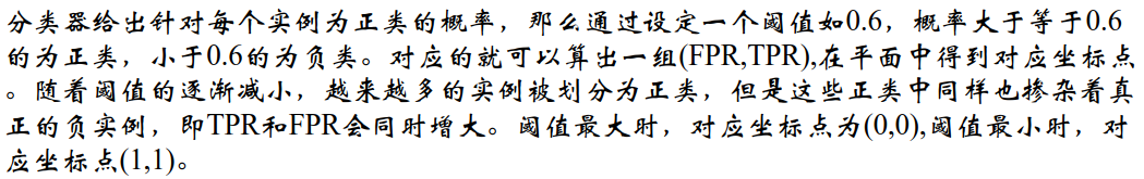
二、分类器性能指标—AUC

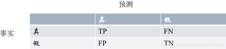
如果想弄懂AUC和ROC曲线，一定要彻底理解混淆矩阵的概念！！！
混淆矩阵中有Postitive(阳性)、Negative(阴性)、False(伪)、True(真)的概念

预测类别为0的为Negative(阴性)，预测类别为1的为Postitive(阳性)
预测错误的为False(伪)、预测正确为True(真)

对上述概念进行组合，就有了混淆矩阵！
在这里插入图片描述

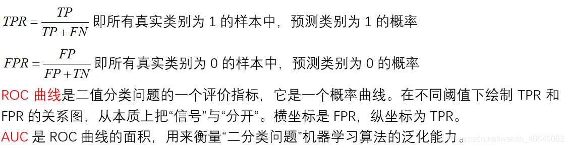
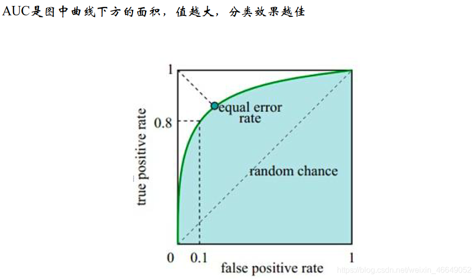
ROC计算过程参见该博客

三、GBDT在流失预警模型中的应用

1.调参过程

导入模块、加载数据集、切分数据集

# 导入模块
import pandas as pd
import numpy as np
from sklearn.ensemble import GradientBoostingClassifier
from sklearn.model_selection import train_test_split, KFold, GridSearchCV
from sklearn import ensemble, metrics

# 读取预处理后的数据集
modelData = pd.read_csv('data/modelData.csv', header=0)
allFeatures = list(modelData.columns)
# 移除CUST_ID与CHURN_CUST_IND列
allFeatures.remove('CUST_ID')
allFeatures.remove('CHURN_CUST_IND')

# 切割数据集
x_train, x_test, y_train, y_test = train_test_split(modelData[allFeatures], modelData['CHURN_CUST_IND'], test_size=0.3,
                                                    shuffle=True)
print(y_train.value_counts())
print(y_test.value_counts())

默认设置的GBDT

# 1.使用默认模型参数
gbdt_0 = GradientBoostingClassifier(random_state=10)
gbdt_0.fit(x_train, y_train)
y_pred = gbdt_0.predict(x_test)
# predict_proba生成一个n行k列的数组，其中n为样本数据量，k为标签个数，
# 每一行为某个样本属于某个标签的概率，每行概率和为1
y_pred_prob = gbdt_0.predict_proba(x_test)[:, 1]
# %g 浮点数字(根据值的大小采用%e或%f)
print('Accuracy : %.4g' % metrics.accuracy_score(y_test, y_pred))
print('AUC(Testing) : %f' % metrics.roc_auc_score(y_test, y_pred_prob))

# 训练集上的accuracy、auc
y_pred_1 = gbdt_0.predict(x_train)
y_pred_prob_1 = gbdt_0.predict_proba(x_train)[:, 1]
print('Accuracy : %.4g' % metrics.accuracy_score(y_train, y_pred_1))
print('AUC(Training) : %f' % metrics.roc_auc_score(y_train, y_pred_prob_1))

调参第一步：
首先从learning rate（步长）和n_estimators（迭代次数）入手。一般是选择一个较小的步长来网格搜索最好的迭代次数。这里，我们不妨将learning rate设置为0.1，迭代次数的所搜次数为20~80，确定下n_estimators（迭代次数）。

# 2.设置一个较小的learning_rate,网格搜索n_estimators
params_test = {
    
    'n_estimators': np.arange(20, 81, 10)}
gbdt_1 = GradientBoostingClassifier(learning_rate=0.1, min_samples_split=300, min_samples_leaf=20,
                                    max_depth=8, max_features='sqrt', subsample=0.8, random_state=10)
gs = GridSearchCV(estimator=gbdt_1, param_grid=params_test, scoring='roc_auc', cv=5)
gs.fit(x_train, y_train)
print('模型最佳参数为', gs.best_params_)
print('模型最好的评分为', gs.best_score_)

模型最佳参数为 {
    
    'n_estimators': 80}
模型最好的评分为 0.9999988452344752

调参第二步：
在学习率与迭代次数确定的情况下，我们开始对决策树进行调参。首先，对决策树最大深度max_depth和内部节点再划分所需最小样本数min_samples_split进行网格搜索，搜索范围分别是3~13和100 ~800。由于内部节点再划分所需最小样本数min_samples_split还与决策树的其他参数存在关联，我们就先确定下决策树最大深度max_depth

# 3.对max_depth与min_samples_split进行网格搜索
params_test = {
    
    'max_depth': np.arange(3, 14, 1), 'min_samples_split': np.arange(100, 801, 100)}
gbdt_2 = GradientBoostingClassifier(learning_rate=0.1, n_estimators=80, min_samples_leaf=20,
                                    max_features='sqrt', subsample=0.8, random_state=10)
gs = GridSearchCV(estimator=gbdt_2, param_grid=params_test, scoring='roc_auc', cv=5)
gs.fit(x_train, y_train)
print('模型最佳参数为', gs.best_params_)
print('模型最好的评分为', gs.best_score_)

调参第三步：

将内部节点再划分所需最小样本数min_samples_split和叶子节点最少样本数min_samples_leaf一起调参。调参范围分别是400-1000以及60-100。

# 4.内部节点再划分所需最小样本数min_samples_split和叶子节点最少样本数min_samples_leaf一起调参
params_test = {
    
    'min_samples_leaf': np.arange(20, 101, 10), 'min_samples_split': np.arange(400, 1001, 100)}
gbdt_3 = GradientBoostingClassifier(learning_rate=0.1, n_estimators=80, max_depth=9,
                                    max_features='sqrt', subsample=0.8, random_state=10)
gs = GridSearchCV(estimator=gbdt_3, param_grid=params_test, scoring='roc_auc', cv=5)
gs.fit(x_train, y_train)
print('模型最佳参数为', gs.best_params_)
print('模型最好的评分为', gs.best_score_)

最终版本

gbdt_4 = GradientBoostingClassifier(learning_rate=0.1, n_estimators=80, max_depth=9, min_samples_leaf=70,
                                    min_samples_split=500, max_features='sqrt', subsample=0.8, random_state=10)
gbdt_4.fit(x_train, y_train)
y_pred_4 = gbdt_4.predict(x_test)
y_pred_prob_4 = gbdt_4.predict_proba(x_test)[:, 1]
print('Accuracy : %.4g' % metrics.accuracy_score(y_test, y_pred_4))
print('AUC(Testing) : %f' % metrics.roc_auc_score(y_test, y_pred_prob_4))

# 训练集上的accuracy、auc
y_pred_1 = gbdt_4.predict(x_train)
y_pred_prob_1 = gbdt_4.predict_proba(x_train)[:, 1]
print('Accuracy : %.4g' % metrics.accuracy_score(y_train, y_pred_1))
print('AUC(Training) : %f' % metrics.roc_auc_score(y_train, y_pred_prob_1))

发现效果竟然还不如默认效果，主要原因是这里我们只使用了0.8的子采样，20%的数据没有参与拟合。
调参第四步：
我们对最大特征数max_features进行网格搜索

# 对max_features进行网格搜索
param_test4 = {
    
    'max_features': range(5, 31, 2)}
gbdt_4 = GradientBoostingClassifier(learning_rate=0.1, n_estimators=80, max_depth=9, min_samples_leaf=70,
                                    min_samples_split=500, subsample=0.8, random_state=10)
gs = GridSearchCV(estimator=gbdt_4, param_grid=param_test4, scoring='roc_auc', cv=5)
gs.fit(x_train, y_train)
print('模型最佳参数为', gs.best_params_)
print('模型最好的评分为', gs.best_score_)

凋参第五步：

# 对subsample进行网格搜索
param_test5 = {
    
    'subsample':[0.6,0.7,0.75,0.8,0.85,0.9]}
gbdt_5 = GradientBoostingClassifier(learning_rate=0.1, n_estimators=80, max_depth=9, min_samples_leaf=70,
                                    min_samples_split=500, max_features=28, random_state=10)
gs = GridSearchCV(estimator=gbdt_5, param_grid=param_test5, scoring='roc_auc', cv=5)
gs.fit(x_train, y_train)
print('模型最佳参数为', gs.best_params_)
print('模型最好的评分为', gs.best_score_)

现在我们已经基本上得到我们所有的调参结果，这时，我们可以减半步长，最大迭代次数加倍来增加我们模型的泛化能力。

2.变量重要性

和随机森林一样，GBDT也可以给出特征的重要性。

clf = GradientBoostingClassifier(learning_rate=0.05, n_estimators=70,max_depth=9, min_samples_leaf =70,
               min_samples_split =1000, max_features=28, random_state=10,subsample=0.8)
clf.fit(X_train, y_train)
importances = clf.feature_importances_
# 按重要性降序对要素进行排序。 默认情况下，argsort返回升序
features_sorted = np.argsort(-importances)
import_feautres = [allFeatures[i] for i in features_sorted]