金融评分卡项目—7.申请评分卡中的数据预处理和特征衍生

文章目录

一、构建信用风险类型的特征

将信息度比较分散的特征综合起来变成信息度比较高的特征。
已经加工成型的信息
表—Master，该表是人维度的信息

idx：每一笔贷款的unique key
UserInfo_*：借款人特征字段
WeblogInfo_*:Info网络行为字段
Education_Info*:学历学籍字段
ThirdParty_Info_PeriodN_*:第三方数据时间段N字段
SocialNetwork_*:社交网络字段
LinstingInfo：借款成交时间
Target：违约标签(1 = 贷款违约，0=正常还款)

1.需要衍生的信息—表1

表—借款人的登录信息，该表是以事件为维度的信息，需要转变成以人为维度的信息

ListingInfo：借款成交时间
LogInfo1：操作代码—类别型
LogInfo2：操作类别—类别型
LogInfo3：登陆时间
idx：每一笔贷款的unique key

时间切片—两个时刻间的跨度
例：申请日期之前30天内的登录次数
基于时间切片进行衍生：
比如：申请日期之前180天内，平均内每月（30天）的登陆次数
常用的时间切片有：（1,2个）月，（1,2个）季度，半年，1年，2年
时间切片的选择：

不能太长：保证大多数样本都能覆盖到
不能太短：丢失信息

如何选择最佳的时间切片？
描述基于不同时间切片所对应的覆盖度，选取覆盖度达到95%的时间切片
在这里插入图片描述
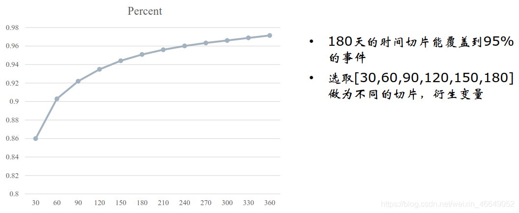
如何选取在最佳时间切片内所衍生的信息？

在该表中，在同一时间切片内，可以衍生的特征有：

操作的次数
不同类别/代码的个数
同一类别/代码的平均操作次数

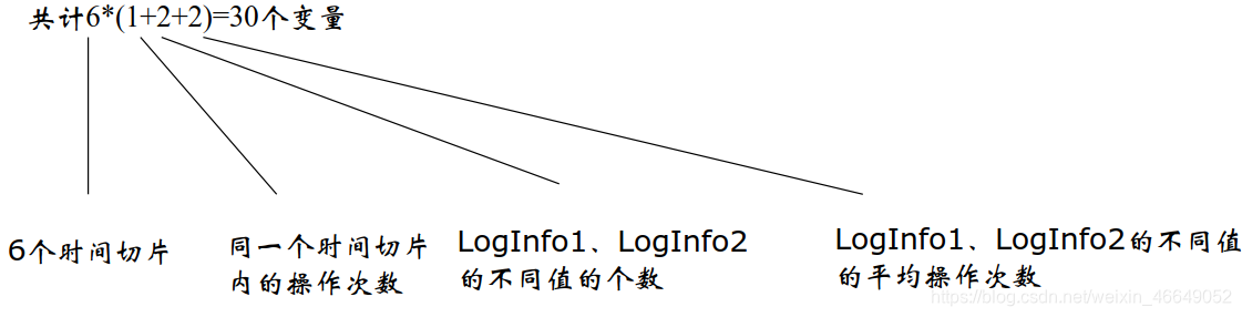
共30个变量。

2.需要衍生的信息—表2

借款人修改信息。该表是以事件为维度的信息，需要转变成以人为维度的信息

ListingInfo1：借款成交时间
UserupdateInfo1：修改内容
UserupdateInfo2：修改时间

特别地，需要做数据预处理

统一大小写
统一Phone、Mobilephone

关注几个特殊变量

是否修改IDNumber（身份证号码）
是否修改Mobilephone（电话号码）
是否修改HASBUYCAR（是否有车）
是否修改MARRIAGESTATUSID（婚姻状况改变）

3.数据清洗

对于类别型变量，

删除缺失率超过50%的变量，剩余变量中的缺失作为一种状态。

对于连续型变量，

删除缺失率超过30%的变量，剩余变量利用随机抽样法对缺失进行补缺；如果使用均值填充的话，最好将极端值剔除掉！
注：在申请评分卡模型中，连续变量中的缺失也可以当成一种状态。

二、特征的分箱

分箱的定义：

将连续变量离散化（组1、组2…）
将多状态的离散变量合并成少状态

分箱的重要性：

稳定性:避免特征中无意义的波动对评分带来的波动
健壮性：避免了极端值的影响

分箱的优势：

可以将缺失作为独立的一个箱代入模型中
将所有变量变换到相似的尺度上

分箱的限制：

计算量大，分箱后需要编码

1.分箱的方法

分箱方法分为有监督与无监督的方法。对于有监督的方法，需要根据目标变量来对变量进行分箱。比如：在流失预警模型中，根据目标变量流失与否来决定收入是如何分箱的

Best—KS
ChiMerge

对于无监督方法，常用的有：等频、等距、聚类（K-means）等

2.监督式分箱法：Best-KS

在这里插入图片描述

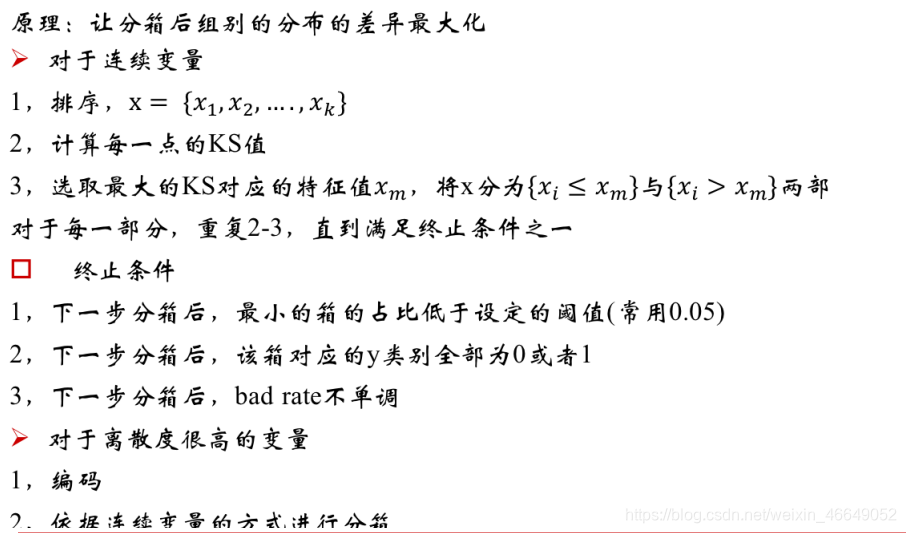
注意：bad rate不单调是一个比较强的条件，当数据质量比较好时，可以用这个

Best-KS的缺陷：

只能针对二分类的情况计算KS

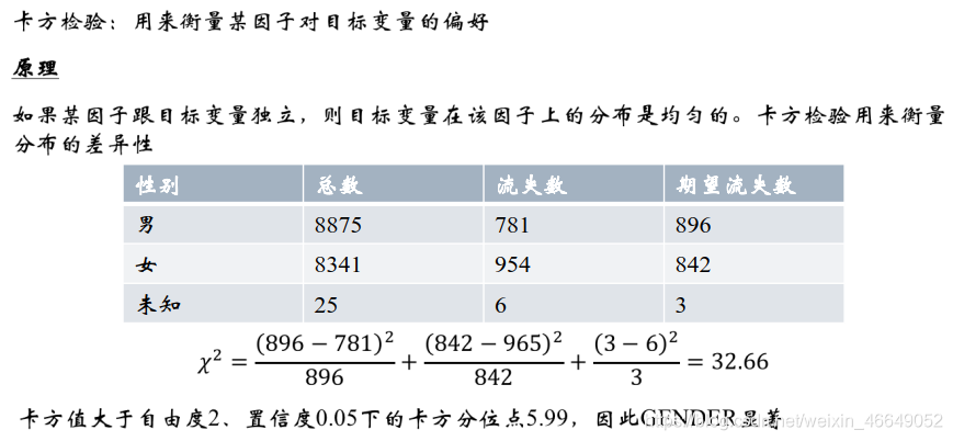
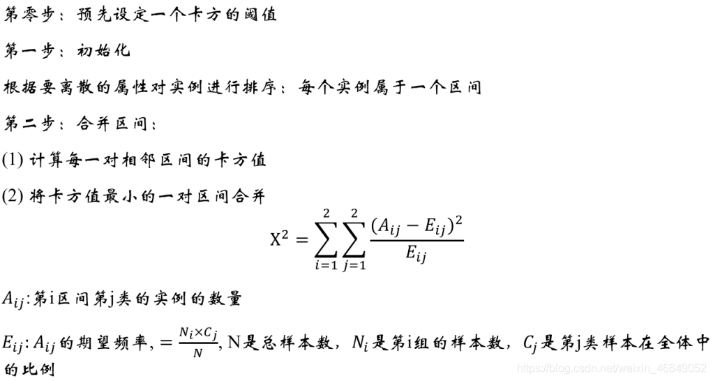
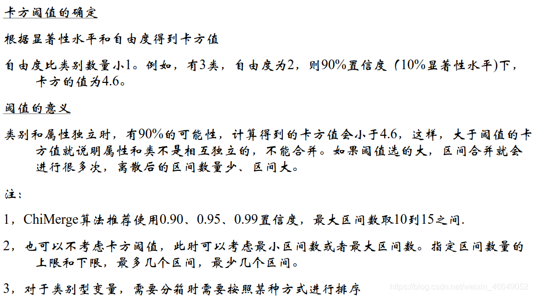
3.卡方分箱法—ChiMerge

卡方分箱法是一种自底向上的数据离散化方法。它依赖于卡方检验：具有最小卡方值的相邻区间合并到一起，直至满足确定的停止准则。基本思想：对于精确的离散化，相对类频率在一个区间内应当完全一致。因此，如果两个相邻的区间具有非常相似的类分布，则这两个区间可以合并；否则，它们应当保持分开（组内的差别很小，组间的差别很大）。而低卡方值表明它们具有相似的类分布。

和Best-KS相比，ChiMerge可以应用到多分类的情况下

组内的差别很小，组间的差别很大。具体到申请评分卡模型中，即组内的逾期率差不多，组间的逾期率差别较大。

在这里插入图片描述

4.无监督分箱方法

无监督的分箱方法是一种不依赖于目标变量的方法。一般有等频、等距、聚类（K-means）分箱
在这里插入图片描述

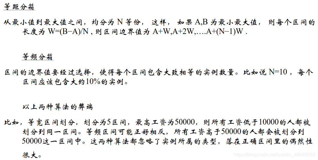
等距与等频是没有理由的，这两种方法完全忽略了目标变量与特征变量（属性）关联度的作用

5.分箱的注意点

对于连续型变量，

使用ChiMerge进行分箱（默认分成5个箱）
检查分箱后的bad rate单调性；倘若不满足，需要进行相邻两箱的合并，直到bad rate单调为止
上述过程是收敛的，因为当箱数为2时，bad rate自然单调
分箱必须覆盖所有训练样本外可能存在的值!
连续性变量，左开右闭

比如收入变量，在训练样本中只有[1004,1008,…1400],[2100,2134,…2500]
但是在测试样本中可能存在1500，此时1500不在任何一个区间，上述划分是有误的。应该[0 ~ 1004],(1004~1400],(1400 ~ 2500]…(10000 ~ 10e9)

对于类别型变量，

当类别数较少时，不需要分箱
当某个或者几个类别的bad rate为0时，需要和最小的非bad rate的箱进行合并
当该变量可以完全区分目标变量时，需要认真检查该变量的合理性
例如：“该申请者在本机构的历史信用行为”把客群的好坏样本完全区分时，需要检查该变量的合理性（有可能是事后变量）

6.多类别离散变量和连续变量的分箱的注意点

多类别离散变量
以bad rate代替原有值，转化成连续型变量再分箱
例：UserInfo_2，原始值有327个城市，分箱后有5个组别

连续型变量
把特殊值单独化为一组
比如：ThirdParty_Info_Period4_1: -1 U [0,1506],-1单独分为一组

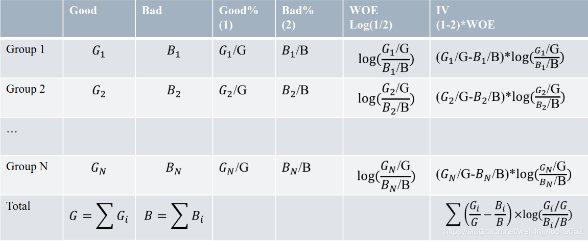
7.特征信息度—IV

IV（Information Value）是衡量特征包含预测变量浓度的一种指标，其恒为正值。
特征信息度：

非负指标
高IV表示该特征和目标变量的关联度高

特征信息度的缺陷：

目标变量只能是二分类
过高的IV，可能有潜在的风险
特征分箱越细，IV越高

常用的阈值：
在这里插入图片描述
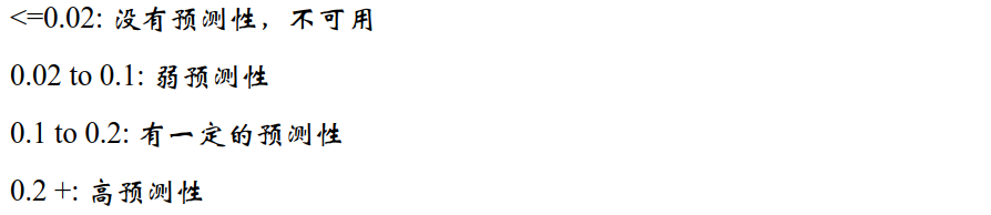
IV最大值不要超过0.8

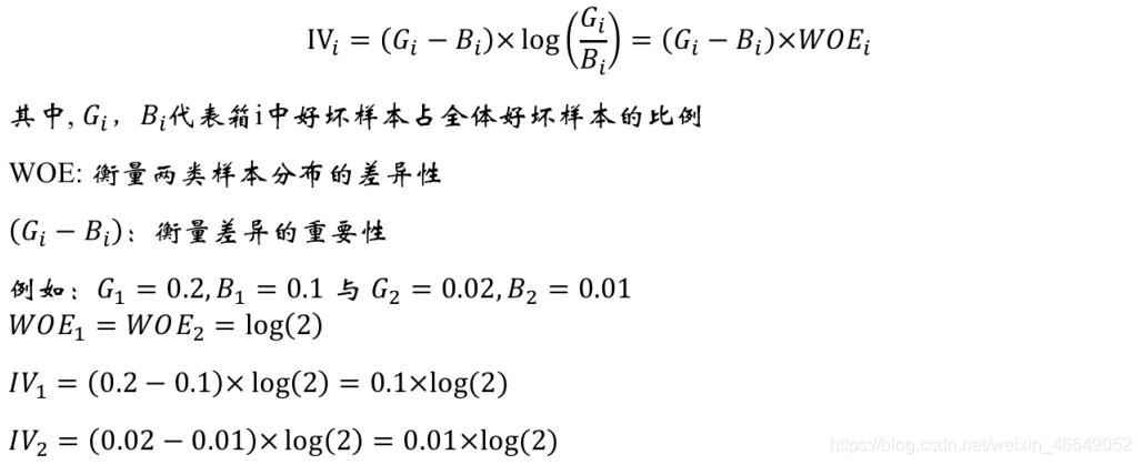
特征信息度的计算：
在这里插入图片描述

特征信息度的作用：

挑选变量

1 .不进行特征挑选，样本矩阵很可能是奇异矩阵(转置×它本身是不可逆的)
2 .变量的维护是有成本的，模型的维护是有成本的。如果能够降低变量的个数，但是仍能保证模型的性能基本不变，降低了模型部署开发的成本。

三、WOE编码

一种有监督的编码方式，将预测类别的集中度的属性作为编码的数值。
优点:

将特征的值规范到相近的尺度上（有正有负，WOE的绝对值波动范围在0.1~3之间）
具有业务意义

缺点：

需要每箱中同时包含好、坏两个类别，由WOE的表达式就可以看得出来

1.计算公式

在这里插入图片描述

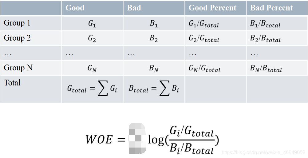
WOE大于0，表明第i组倾向于出现好的
WOE小于0，表明第i组倾向于出现坏的

2.WOE编码的意义

符号与好样本的比例相关

WOE大于0，表明第i组倾向于出现好的
WOE小于0，表明第i组倾向于出现坏的
要求回归模型的系数为负

四、信用风险中的变量分析

1.单变量分析

单变量分析主要考虑的是特征与目标变量的关联度以及特征自身的一些情况。以分箱后的WOE为值

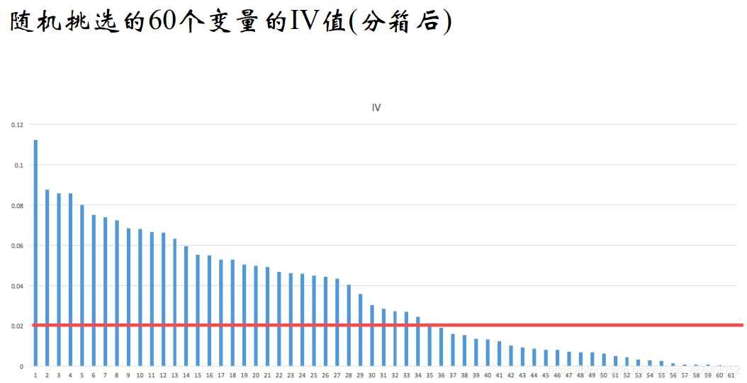
用IV检验有效性,IV不能低于0.02
连续变量bad rate的单调性（可以放宽到U型）

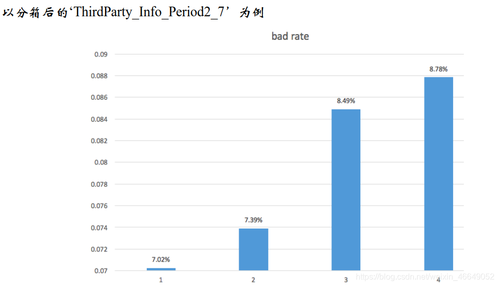
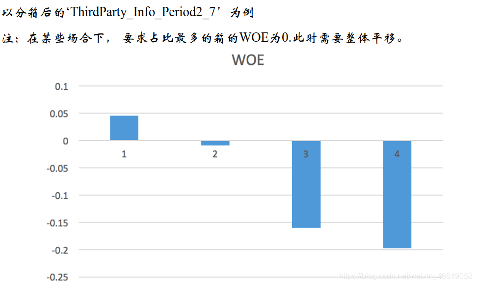
bad rate 与WOE的趋势一致
当然也有可能不一样，毕竟公式不一样
bad rate = B_i / (B_i + G_i)
单一区间的占比不宜过高

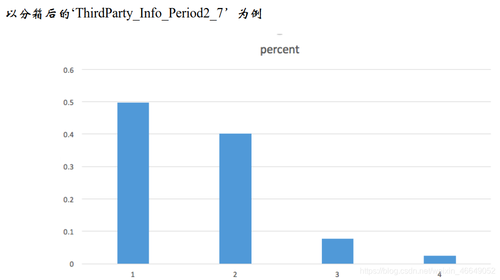
要求是占比最高的不超过90%（常用）或者占比最少的不低于5%,满足一项即可

2.多变量分析

多变量分析主要是为了避免共线性对建模造成的影响，同时，也实现了降维。
变量的两两相关性：
当变量之间相关性高时，只能保留一个

可以选择IV高的
可以选择分箱均衡的

WOE相关性矩阵：
在这里插入图片描述
多变量分析—变量之间的多重共线性：

当某个变量的VIF超过10，需要逐一删除解释变量。当删除掉x_k时，发现VIF低于10，从{x_k,x_i}中删除掉IV较低的一个。

五、操作步骤总结

读取csv文件，并检查Idx的一致性

为了方便后续缺失值操作，一般先将表中代表缺失值的东西替换为np.nan
对表—借款人登录信息与借款人修改信息进行特征衍生

1 .查看不同时间切片的复杂度，选择复杂度大于95%的时间切片，这就是最大的时间窗口
2.以人为维度，分别统计每个Idx的总操作次数、总操作类数，每一类的平均操作次数,并且关注其中的特别变量
对连续型变量与类别型变量填充缺失值

删除缺失率超过50%的类别变量，剩余变量缺失作为一种状态
删除缺失率超过30%的连续型变量，剩余变量利用随机抽样法对缺失值进行补缺
对连续型变量与类别型变量进行卡方分箱

对于类别型变量，按照下列步骤:
1.如果变量的唯一值超过5个，我们就需要分箱；计算bad rate，并以bad rate对变量进行编码，按照bad rate进行排序，计算每一对相邻区间的卡方值，将卡方值最小的区间进行合并,直至分箱数为5
2.另外,
2.1 检查占比最高的组，如果有一组占比超过95%（90%），则删除该变量(占比高相当于常量型特征)
2.2 检查每一个分箱的bad rate，当某个或者几个类别的bad rate为0时，需要和最小的非bad rate的箱进行合并

对于连续型变量，我们需要做如下工作：
1.按ChiMerge拆分变量（默认分为5个bin）
2.检查bate rate，如果不是单调的话，我们减少箱数，直到bate rate是单调
3.如果最大bin占用超过90％，则删除变量

选择IV大于0.02的变量，并进行WOE编码
单因子分析与多因子分析

单因子分析，经过上述步骤就以满足
多因子分析，变量两两间具有相关性，则选择IV值大的变量

六、代码

写法规范：将自定义函数与主程序分开，将专门书写自定义函数的程序写入路径（增加到系统路径），然后在主程序里import
自定义函数文件

#!usr/bin/env python
# -*- coding:utf-8 -*-
"""
@author: admin
@file: scoredcard_functions.py
@time: 2021/03/11
@desc:
"""
import random
import pandas as pd
import numpy as np


def timeWindowSelection(df, daysCol, time_windows):
    """
    计算每一个时间切片内的事件的累积频率
    :param df: 数据集
    :param daysCol:时间间隔
    :param time_windows:时间窗口列表
    :return:返回覆盖度
    """
    freq_tw = {
    
    }
    for tw in time_windows:
        freq = sum(df[daysCol].apply(lambda x: int(x <= tw)))
        freq_tw[tw] = freq / df[daysCol].shape[0]
    return freq_tw


def ChangeContent(x):
    """
    数据预处理：统一大小写、统一_PHONE与_MOBILEPHONE
    :param x: UserupdateInfo1列字符
    :return:返回处理后的字符
    """
    y = x.upper()
    if y == '_MOBILEPHONE':
        y = '_PHONE'
    return y


def missingCategorical(df, x):
    """
    计算类别型变量的缺失比例
    :param df: 数据集
    :param x: 类别型变量
    :return: 返回缺失比例
    """
    missing_vals = df[x].map(lambda x: int(x != x))
    return sum(missing_vals) * 1.0 / df.shape[0]


def missingContinuous(df, x):
    """
    计算连续型变量的缺失比例
    :param df:
    :param x:
    :return:
    """
    missing_vals = df[x].map(lambda x: int(np.isnan(x)))
    return sum(missing_vals) * 1.0 / df.shape[0]


def makeUpRandom(x, sampledList):
    """
    对于连续型变量，利用随机抽样法补充缺失值
    :param x:连续型变量的值
    :param sampledList:随机抽样的列表
    :return:补缺后的值
    """
    # 非缺失，直接返回；缺失，填充后返回
    if x == x:
        return x
    else:
        return random.sample(sampledList, 1)


def AssignBin(x, cutOffPoints):
    '''
    设置使得分箱覆盖所有训练样本外可能存在的值
    :param x: the value of variable
    :param cutOffPoints: the ChiMerge result for continous variable连续变量的卡方分箱结果
    :return: bin number, indexing from 0
    for example, if cutOffPoints = [10,20,30], if x = 7, return Bin 0. If x = 35, return Bin 3
    即将cutOffPoints = [10,20,30]分为4段，[0,10],(10,20],(20,30],(30,30+]
    '''
    numBin = len(cutOffPoints) + 1
    if x <= cutOffPoints[0]:
        return 'Bin 0'
    elif x > cutOffPoints[-1]:
        return 'Bin {}'.format(numBin - 1)
    else:
        for i in range(0, numBin - 1):
            if cutOffPoints[i] < x <= cutOffPoints[i + 1]:
                return 'Bin {}'.format(i + 1)


def MaximumBinPcnt(df, col):
    """
    :param df:
    :param col:
    :return:
    """
    N = df.shape[0]
    total = df.groupby([col])[col].count()
    pcnt = total * 1.0 / N
    return max(pcnt)


def CalcWOE(df, col, target):
    '''
    计算WOE
    :param df: dataframe containing feature and target
    :param col: 需要计算WOE与IV的特征变量，通常是类别型变量
    :param target: 目标变量
    :return: WOE and IV in a dictionary
    '''
    total = df.groupby([col])[target].count()
    total = pd.DataFrame({
    
    'total': total})
    bad = df.groupby([col])[target].sum()
    bad = pd.DataFrame({
    
    'bad': bad})
    regroup = total.merge(bad, left_index=True, right_index=True, how='left')
    regroup.reset_index(level=0, inplace=True)
    # 总数量
    N = sum(regroup['total'])
    # 坏的数量
    B = sum(regroup['bad'])
    regroup['good'] = regroup['total'] - regroup['bad']
    # 好的数量
    G = N - B
    regroup['bad_pcnt'] = regroup['bad'].map(lambda x: x * 1.0 / B)
    regroup['good_pcnt'] = regroup['good'].map(lambda x: x * 1.0 / G)
    regroup['WOE'] = regroup.apply(lambda x: np.log(x.good_pcnt * 1.0 / x.bad_pcnt), axis=1)
    # 计算WOE
    WOE_dict = regroup[[col, 'WOE']].set_index(col).to_dict(orient='index')
    # 计算IV
    IV = regroup.apply(lambda x: (x.good_pcnt - x.bad_pcnt) * np.log(x.good_pcnt * 1.0 / x.bad_pcnt), axis=1)
    IV = sum(IV)
    return {
    
    "WOE": WOE_dict, 'IV': IV}


def BadRateEncoding(df, col, target):
    '''
    bad rate编码
    :param df: dataframe containing feature and target
    :param col: 需要以bad rate进行编码的特征变量，通常是类别型变量
    :param target: good/bad indicator
    :return: 返回被bad rate编码的类别型变量
    '''
    total = df.groupby([col])[target].count()
    total = pd.DataFrame({
    
    'total': total})
    bad = df.groupby([col])[target].sum()
    bad = pd.DataFrame({
    
    'bad': bad})
    regroup = total.merge(bad, left_index=True, right_index=True, how='left')
    regroup.reset_index(level=0, inplace=True)
    regroup['bad_rate'] = regroup.apply(lambda x: x.bad * 1.0 / x.total, axis=1)
    br_dict = regroup[[col, 'bad_rate']].set_index([col]).to_dict(orient='index')
    badRateEnconding = df[col].map(lambda x: br_dict[x]['bad_rate'])
    return {
    
    'encoding': badRateEnconding, 'br_rate': br_dict}


def Chi2(df, total_col, bad_col, overallRate):
    '''
    # 计算卡方值
    :param df: the dataset containing the total count and bad count
    :param total_col: total count of each value in the variable
    :param bad_col: bad count of each value in the variable
    :param overallRate: the overall bad rate of the training set—逾期率
    :return: the chi-square value
    '''
    df2 = df.copy()
    df2['expected'] = df[total_col].apply(lambda x: x * overallRate)
    combined = zip(df2['expected'], df2[bad_col])
    chi = [(i[0] - i[1]) ** 2 / i[0] for i in combined]
    chi2 = sum(chi)
    return chi2


def AssignGroup(x, bin):
    """
    将超过100个的属性值调整到100个
    :param x: 属性值
    :param bin: 99个分割点
    :return: 调整后的值
    """
    N = len(bin)
    if x <= min(bin):
        return min(bin)
    elif x > max(bin):
        return 10e10
    else:
        for i in range(N - 1):
            if bin[i] < x <= bin[i + 1]:
                return bin[i + 1]


# ChiMerge_MaxInterval:
def ChiMerge_MaxInterval_Original(df, col, target, max_interval=5):
    '''
    通过指定最大分箱数，使用卡方值拆分连续变量
    :param df: the dataframe containing splitted column, and target column with 1-0
    :param col: splitted column
    :param target: target column with 1-0
    :param max_interval: 最大分箱数
    :return: the combined bins
    '''
    colLevels = set(df[col])
    # since we always combined the neighbours of intervals, we need to sort the attributes
    # 排序
    colLevels = sorted(list(colLevels))
    N_distinct = len(colLevels)
    if N_distinct <= max_interval:
        print("The number of original levels for {} is less than or equal to max intervals".format(col))
        return colLevels[:-1]
    else:
        # Step 1: group the dataset by col and work out the total count & bad count in each level of the raw column
        # 按col对数据集进行分组，并计算出total count & bad count
        total = df.groupby([col])[target].count()
        total = pd.DataFrame({
    
    'total': total})
        bad = df.groupby([col])[target].sum()
        bad = pd.DataFrame({
    
    'bad': bad})
        regroup = total.merge(bad, left_index=True, right_index=True, how='left')
        # 重置索引，将原来的index变为数据列保留下来
        regroup.reset_index(level=0, inplace=True)
        N = sum(regroup['total'])
        B = sum(regroup['bad'])
        # the overall bad rate will be used in calculating expected bad count
        # 总的逾期率
        overallRate = B * 1.0 / N
        # 每一个属性属于一个区间
        groupIntervals = [[i] for i in colLevels]
        groupNum = len(groupIntervals)
        # 终止条件：在迭代的每个步骤中，间隔数等于预先指定的阈值（最大分箱数），我们计算每个属性的卡方值
        while (len(groupIntervals) > max_interval):
            chisqList = []
            for interval in groupIntervals:
                df2 = regroup.loc[regroup[col].isin(interval)]
                chisq = Chi2(df2, 'total', 'bad', overallRate)
                chisqList.append(chisq)
            # 找到最小卡方值的位置，并将该卡方值与左右两侧相邻的较小的卡方值合并
            min_position = chisqList.index(min(chisqList))
            if min_position == 0:
                combinedPosition = 1
            elif min_position == groupNum - 1:
                combinedPosition = min_position - 1
            else:
                if chisqList[min_position - 1] <= chisqList[min_position + 1]:
                    combinedPosition = min_position - 1
                else:
                    combinedPosition = min_position + 1
            groupIntervals[min_position] = groupIntervals[min_position] + groupIntervals[combinedPosition]
            # after combining two intervals, we need to remove one of them
            groupIntervals.remove(groupIntervals[combinedPosition])
            groupNum = len(groupIntervals)
        groupIntervals = [sorted(i) for i in groupIntervals]
        cutOffPoints = [i[-1] for i in groupIntervals[:-1]]
        return cutOffPoints


def ChiMerge_MaxInterval(df, col, target, max_interval=5):
    '''
    通过指定最大分箱数，使用卡方值拆分连续变量
    :param df: the dataframe containing splitted column, and target column with 1-0
    :param col: splitted column
    :param target: target column with 1-0
    :param max_interval: 最大分箱数
    :return: 返回分箱点
    '''
    colLevels = sorted(list(set(df[col])))
    N_distinct = len(colLevels)
    if N_distinct <= max_interval:
        print("The number of original levels for {} is less than or equal to max intervals".format(col))
        return colLevels[:-1]
    else:
        # 如果属性过多，则时间代价较大，不妨取100个属性进行分箱
        if N_distinct > 100:
            ind_x = [int(i / 100.0 * N_distinct) for i in range(1, 100)]
            split_x = [colLevels[i] for i in ind_x]
            df['temp'] = df[col].map(lambda x: AssignGroup(x, split_x))
        else:
            df['temp'] = df[col]
        # Step 1: group the dataset by col and work out the total count & bad count in each level of the raw column
        # 按col对数据集进行分组，并计算出total count & bad count
        total = df.groupby(['temp'])[target].count()
        total = pd.DataFrame({
    
    'total': total})
        bad = df.groupby(['temp'])[target].sum()
        bad = pd.DataFrame({
    
    'bad': bad})
        regroup = total.merge(bad, left_index=True, right_index=True, how='left')
        regroup.reset_index(level=0, inplace=True)
        N = sum(regroup['total'])
        B = sum(regroup['bad'])
        # the overall bad rate will be used in calculating expected bad count
        # 计算总的逾期率
        overallRate = B * 1.0 / N
        # initially, each single attribute forms a single interval
        # since we always combined the neighbours of intervals, we need to sort the attributes
        colLevels = sorted(list(set(df['temp'])))
        groupIntervals = [[i] for i in colLevels]
        groupNum = len(groupIntervals)
        # 终止条件：在迭代的每个步骤中，间隔数等于预先指定的阈值（最大分箱数），我们计算每个属性的卡方值
        while (len(groupIntervals) > max_interval):
            chisqList = []
            for interval in groupIntervals:
                df2 = regroup.loc[regroup['temp'].isin(interval)]
                chisq = Chi2(df2, 'total', 'bad', overallRate)
                chisqList.append(chisq)
            # 找到最小卡方值的位置，并将该卡方值与左右两侧相邻的较小的卡方值合并
            min_position = chisqList.index(min(chisqList))
            if min_position == 0:
                combinedPosition = 1
            elif min_position == groupNum - 1:
                combinedPosition = min_position - 1
            else:
                if chisqList[min_position - 1] <= chisqList[min_position + 1]:
                    combinedPosition = min_position - 1
                else:
                    combinedPosition = min_position + 1
            groupIntervals[min_position] = groupIntervals[min_position] + groupIntervals[combinedPosition]
            # after combining two intervals, we need to remove one of them
            groupIntervals.remove(groupIntervals[combinedPosition])
            groupNum = len(groupIntervals)
        groupIntervals = [sorted(i) for i in groupIntervals]
        # 取最大的点
        cutOffPoints = [i[-1] for i in groupIntervals[:-1]]
        del df['temp']
        return cutOffPoints


def BadRateMonotone(df, sortByVar, target):
    """
    分成5个箱后，判断bad rate是否是单调的，可以是单调上升，也可以是单调下降；如果不单调的话，继续合并
    :param df: DataFrame
    :param sortByVar:分箱后的变量
    :param target:目标变量
    :return: 返回是否单调
    """
    df2 = df.sort([sortByVar])
    total = df2.groupby([sortByVar])[target].count()
    total = pd.DataFrame({
    
    'total': total})
    bad = df2.groupby([sortByVar])[target].sum()
    bad = pd.DataFrame({
    
    'bad': bad})
    regroup = total.merge(bad, left_index=True, right_index=True, how='left')
    regroup.reset_index(level=0, inplace=True)
    combined = zip(regroup['total'], regroup['bad'])
    badRate = [x[1] * 1.0 / x[0] for x in combined]

    badRateMonotone = [badRate[i] < badRate[i + 1] for i in range(len(badRate) - 1)]
    Monotone = len(set(badRateMonotone))
    if Monotone == 1:
        return True
    else:
        return False



def MergeBad0(df, col, target):
    '''
    当某个或者几个类别的bad rate为0时，需要和最小的非bad rate的箱进行合并
     :param df: dataframe containing feature and target
     :param col: the feature that needs to be calculated the WOE and iv, usually categorical type
     :param target: good/bad indicator
     :return: WOE and IV in a dictionary
     '''
    total = df.groupby([col])[target].count()
    total = pd.DataFrame({
    
    'total': total})
    bad = df.groupby([col])[target].sum()
    bad = pd.DataFrame({
    
    'bad': bad})
    regroup = total.merge(bad, left_index=True, right_index=True, how='left')
    regroup.reset_index(level=0, inplace=True)
    regroup['bad_rate'] = regroup.apply(lambda x: x.bad * 1.0 / x.total, axis=1)
    # 按bad rate列进行排序
    regroup = regroup.sort_values(by='bad_rate')
    col_regroup = [[i] for i in regroup[col]]
    for i in range(regroup.shape[0]):
        col_regroup[1] = col_regroup[0] + col_regroup[1]
        col_regroup.pop(0)
        if regroup['bad_rate'][i + 1] > 0:
            break
    newGroup = {
    
    }
    for i in range(len(col_regroup)):
        for g2 in col_regroup[i]:
            newGroup[g2] = 'Bin ' + str(i)
    return newGroup

主程序

#!usr/bin/env python
# -*- coding:utf-8 -*-
"""
@author: admin
@file: scorecard model features.py
@time: 2021/03/11
@desc:
"""
import pandas as pd
import datetime
import collections
import numpy as np
import numbers
import random
from pandas.plotting import scatter_matrix
from sklearn.linear_model import LinearRegression
from itertools import combinations
# 添加系统路径
import sys

sys.path.append(r"D:/PycharmProjects/Work preparation/九、人工智能项目班/scoredcard/")
from scoredcard_functions import *

# step0:读取csv文件，检查Idx的一致性
data1 = pd.read_csv('data/PPD_LogInfo_3_1_Training_Set.csv', header=0)
data2 = pd.read_csv('data/PPD_Training_Master_GBK_3_1_Training_Set.csv', header=0, encoding='gbk')
data3 = pd.read_csv('data/PPD_Userupdate_Info_3_1_Training_Set.csv', header=0)
data1_Idx, data2_Idx, data3_Idx = set(data1.Idx), set(data2.Idx), set(data3.Idx)
check_Idx_integrity = (data1_Idx - data2_Idx) | (data2_Idx - data1_Idx) | (data1_Idx - data3_Idx) | (
        data3_Idx - data1_Idx)
# 将空替换为np.NaN
data1.replace('', np.nan, inplace=True)
data2.replace('', np.nan, inplace=True)
data3.replace('', np.nan, inplace=True)

# step1:PPD_LogInfo_3_1_Training_Set 和 PPD_Userupdate_Info_3_1_Training_Set数据集的特征衍生
# 先对PPD_LogInfo_3_1_Training_Set数据集进行特征衍生
# 提取每一个申请人的申请时间间隔
# 登陆时间
data1['logInfo'] = data1['LogInfo3'].map(lambda x: datetime.datetime.strptime(x, '%Y-%m-%d'))
# 借款成交时间
data1['Listinginfo'] = data1['Listinginfo1'].map(lambda x: datetime.datetime.strptime(x, '%Y-%m-%d'))
# 借款成交时间-登陆时间
data1['ListingGap'] = data1[['logInfo', 'Listinginfo']].apply(lambda x: (x[1] - x[0]).days, axis=1)
# 查看不同时间切片的覆盖度，发现180天时，覆盖度达到95%
timeWindows = timeWindowSelection(data1, 'ListingGap', range(30, 361, 30))
print(timeWindows)

# 我们将时间窗口设置为[7,30,60,90,120,150,180]，在不同时间切片内衍生变量
time_window = [7, 30, 60, 90, 120, 150, 180]
# 可以衍生特征
var_list = ['LogInfo1', 'LogInfo2']
# drop_duplicates()表示去除重复项
data1GroupbyIdx = pd.DataFrame({
    
    'Idx': data1['Idx'].drop_duplicates()})
for tw in time_window:
    data1['TruncatedLogInfo'] = data1['Listinginfo'].map(lambda x: x + datetime.timedelta(-tw))  # timedelta第一个参数为day
    # 在时间间隔内的数据
    temp = data1.loc[data1['logInfo'] >= data1['TruncatedLogInfo']]
    for var in var_list:
        # count the frequences of LogInfo1 and LogInfo2——操作的次数
        count_stats = temp.groupby(['Idx'])[var].count().to_dict()
        data1GroupbyIdx[str(var) + '_' + str(tw) + '_count'] = data1GroupbyIdx['Idx'].map(
            lambda x: count_stats.get(x, 0))

        # count the distinct value of LogInfo1 and LogInfo2——不同操作类别/代码的个数
        Idx_UserupdateInfo1 = temp[['Idx', var]].drop_duplicates()
        uniq_stats = Idx_UserupdateInfo1.groupby(['Idx'])[var].count().to_dict()

        data1GroupbyIdx[str(var) + '_' + str(tw) + '_unique'] = data1GroupbyIdx['Idx'].map(
            lambda x: uniq_stats.get(x, 0))

        # calculate the average count of each value in LogInfo1 and LogInfo2—计算同一类别/代码的平均操作次数
        data1GroupbyIdx[str(var) + '_' + str(tw) + '_avg_count'] = data1GroupbyIdx[
            [str(var) + '_' + str(tw) + '_count', str(var) + '_' + str(tw) + '_unique']]. \
            apply(lambda x: x[0] * 1.0 / x[1], axis=1)

# 对PPD_Userupdate_Info_3_1_Training_Set数据集进行特征衍生
# 借款成交日期
data3['ListingInfo'] = data3['ListingInfo1'].map(lambda x: datetime.datetime.strptime(x, '%Y/%m/%d'))
# 借款人修改时间
data3['UserupdateInfo'] = data3['UserupdateInfo2'].map(lambda x: datetime.datetime.strptime(x, '%Y/%m/%d'))
# 时间间隔 = 借款成交日期 - 借款人修改时间
data3['ListingGap'] = data3[['UserupdateInfo', 'ListingInfo']].apply(lambda x: (x[1] - x[0]).days, axis=1)
# collections.Counter表示计算“可迭代序列中”各个元素（element）的数量
collections.Counter(data3['ListingGap'])
# np.histogram()是一个生成直方图的函数
# np.histogram() 默认地使用10个相同大小的区间（箱），然后返回一个元组（频数，分箱的边界）
hist_ListingGap = np.histogram(data3['ListingGap'])
hist_ListingGap = pd.DataFrame({
    
    'Freq': hist_ListingGap[0], 'gap': hist_ListingGap[1][1:]})
# 频数累加
hist_ListingGap['CumFreq'] = hist_ListingGap['Freq'].cumsum()
# 频数的百分比
hist_ListingGap['CumPercent'] = hist_ListingGap['CumFreq'].map(lambda x: x * 1.0 / hist_ListingGap.iloc[-1]['CumFreq'])
# 我们将时间窗口设置为[7,30,60,90,120,150,180]，在不同时间切片内衍生变量
# 数据预处理:统一大小写、统一Phone、Mobilephone
data3['UserupdateInfo1'] = data3['UserupdateInfo1'].map(ChangeContent)
# 去掉重复索引，添加衍生变量
data3GroupbyIdx = pd.DataFrame({
    
    'Idx': data3['Idx'].drop_duplicates()})
time_window = [7, 30, 60, 90, 120, 150, 180]

for tw in time_window:
    # 时间切片范围内的数据
    data3['TruncatedLogInfo'] = data3['ListingInfo'].map(lambda x: x + datetime.timedelta(-tw))
    temp = data3.loc[data3['UserupdateInfo'] >= data3['TruncatedLogInfo']]

    # 统计每个Idx的操作次数
    freq_stats = temp.groupby(['Idx'])['UserupdateInfo1'].count().to_dict()
    data3GroupbyIdx['UserupdateInfo_' + str(tw) + '_freq'] = data3GroupbyIdx['Idx'].map(lambda x: freq_stats.get(x, 0))

    # 统计每个Idx的操作类数
    Idx_UserupdateInfo1 = temp[['Idx', 'UserupdateInfo1']].drop_duplicates()
    # print(Idx_UserupdateInfo1)
    unique_stats = Idx_UserupdateInfo1.groupby(['Idx'])['UserupdateInfo1'].count().to_dict()
    data3GroupbyIdx['UserupdateInfo_' + str(tw) + '_unique'] = data3GroupbyIdx['Idx'].map(
        lambda x: unique_stats.get(x, x))

    # 统计每个Idx每个操作类型的平均操作次数
    data3GroupbyIdx['UserupdateInfo_' + str(tw) + '_avg_count'] = data3GroupbyIdx[
        ['UserupdateInfo_' + str(tw) + '_freq', 'UserupdateInfo_' + str(tw) + '_unique']]. \
        apply(lambda x: x[0] * 1.0 / x[1], axis=1)

    # whether the applicant changed items like IDNUMBER,HASBUYCAR, MARRIAGESTATUSID, PHONE
    # 关注特殊变量——是否修改了这些变量
    Idx_UserupdateInfo1['UserupdateInfo1'] = Idx_UserupdateInfo1['UserupdateInfo1'].map(lambda x: [x])
    # 相加
    Idx_UserupdateInfo1_V2 = Idx_UserupdateInfo1.groupby(['Idx'])['UserupdateInfo1'].sum()
    for item in ['_IDNUMBER', '_HASBUYCAR', '_MARRIAGESTATUSID', '_PHONE']:
        item_dict = Idx_UserupdateInfo1_V2.map(lambda x: int(item in x)).to_dict()
        # print(item_dict)
        data3GroupbyIdx['UserupdateInfo_' + str(tw) + str(item)] = data3GroupbyIdx['Idx'].map(
            lambda x: item_dict.get(x, x))

allData = pd.concat([data2.set_index('Idx'), data3GroupbyIdx.set_index('Idx'), data1GroupbyIdx.set_index('Idx')],
                    axis=1)
allData.to_csv('allData_0.csv', encoding='gbk')

# step2:Makeup missing value for categorical variables and continuous variables
# 为类别变量与连续型变量填充缺失值

allData = pd.read_csv('allData_0.csv', header=0, encoding='gbk')
allFeatures = list(allData.columns)
# 移除借款成交时间与目标变量
allFeatures.remove('ListingInfo')
allFeatures.remove('target')
allFeatures.remove('Idx')

# 删除常量型特征
for col in allFeatures:
    if len(set(allData[col])) == 1:
        allFeatures.remove(col)

# 将自变量分为连续型变量与类别型变量
numerical_var = []
for var in allFeatures:
    uniq_vals = list(set(allData[var]))
    if np.nan in uniq_vals:
        uniq_vals.remove(np.nan)
    if len(uniq_vals) >= 10 and isinstance(uniq_vals[0], numbers.Real):
        numerical_var.append(var)

categorical_var = [i for i in allFeatures if i not in numerical_var]

# 删除缺失率超过50%的类别变量，剩余变量缺失作为一种状态
missing_pcnt_threshould_1 = 0.5
for var in categorical_var:
    missingRate = missingCategorical(allData, var)
    print(var, ' has missing rate as ', missingRate)
    if missingRate > missing_pcnt_threshould_1:
        categorical_var.remove(var)
        del allData[var]
    if 0 < missingRate < missing_pcnt_threshould_1:
        allData[var] = allData[var].map(lambda x: "'" + str(x) + "'")

# 删除缺失率超过30%的连续型变量，剩余变量利用随机抽样法对缺失值进行补缺
missing_pcnt_threshould_2 = 0.3
for var in numerical_var:
    missingRate = missingContinuous(allData, var)
    if missingRate > missing_pcnt_threshould_2:
        numerical_var.remove(var)
        del allData[var]
        print('we delete variable {} because of its high missing rate'.format(var))
    else:
        if missingRate > 0:
            not_missing = allData.loc[allData[var] == allData[var]][var]
            # Population must be a sequence or set.  For dicts, use list(d)
            allData[var] = allData[var].map(lambda x: makeUpRandom(x, list(not_missing)))
allData.to_csv('allData_1.csv', header=True, encoding='gbk', columns=allData.columns, index=False)

# step3:变量分箱
# 对于每个类别变量，如果其唯一值大于5，我们将使用ChiMerge对其进行合并
trainData = pd.read_csv('allData_1.csv', header=0, encoding='gbk')
allFeatures = list(trainData.columns)
allFeatures.remove('ListingInfo')
allFeatures.remove('target')
allFeatures.remove('Idx')
# 数据预处理—将类别变量中大写转化成小写
for col in categorical_var:
    trainData[col] = trainData[col].map(lambda x: str(x).upper())

"""
对于类别型变量，按照下列步骤:
1.如果变量的唯一值超过5个，我们就需要分箱；计算bad rate，并以bad rate对变量进行编码，按照bad rate进行排序，计算每一对相邻区间的卡方值，
将卡方值最小的区间进行合并
2.另外,
    2.1 检查占比最高的组，如果有一组占比超过95%（90%），则删除该变量(占比高相当于常量型特征)
    2.2 检查每一个分箱的bad rate，当某个或者几个类别的bad rate为0时，需要和最小的非bad rate的箱进行合并
"""
deleted_features = []  # delete the categorical features in one of its single bin occupies more than 90%
encoded_features = []
merged_features = []
var_IV = {
    
    }  # save the IV values for binned features
WOE_dict = {
    
    }
for col in categorical_var:
    print('we are processing {}'.format(col))
    if len(set(trainData[col])) > 5:
        print('{} is encoded with bad rate'.format(col))
        col0 = str(col) + '_encoding'
        trainData[col0] = BadRateEncoding(trainData, col, 'target')['encoding']
        # 当做连续型变量
        numerical_var.append(col0)
        encoded_features.append(col0)
        del trainData[col]
    else:
        maxPcnt = MaximumBinPcnt(trainData, col)
        if maxPcnt > 0.9:
            print('{} is deleted because of large percentage of single bin'.format(col))
            deleted_features.append(col)
            categorical_var.remove(col)
            del trainData[col]
            continue
        bad_bin = trainData.groupby([col])['target'].sum()
        if min(bad_bin) == 0:
            print('{} has 0 bad sample!'.format(col))
            # 当某个或者几个类别的bad rate为0时，需要和最小的非bad rate的箱进行合并
            mergeBin = MergeBad0(trainData, col, 'target')
            col1 = str(col) + '_mergeByBadRate'
            trainData[col1] = trainData[col].map(mergeBin)
            # 计算合并后组的最大占比
            maxPcnt = MaximumBinPcnt(trainData, col1)
            if maxPcnt > 0.9:
                print('{} is deleted because of large percentage of single bin'.format(col))
                deleted_features.append(col)
                categorical_var.remove(col)
                del trainData[col]
                continue
            WOE_IV = CalcWOE(trainData, col1, 'target')
            WOE_dict[col1] = WOE_IV['WOE']
            var_IV[col1] = WOE_IV['IV']
            merged_features.append(col)
            del trainData[col]
        else:
            WOE_IV = CalcWOE(trainData, col, 'target')
            WOE_dict[col] = WOE_IV['WOE']
            var_IV[col] = WOE_IV['IV']

"""
对于连续型变量，我们需要做如下工作：
1.按ChiMerge拆分变量（默认分为5个bin）
2.检查bate rate，如果不是单调的话，我们减少箱数，直到bate rate是单调
3.如果最大bin占用超过90％，则删除变量
"""
for col in numerical_var:
    print("{} is in processing".format(col))
    col1 = str(col) + '_Bin'
    # 卡方分箱，返回分箱点
    cutOffPoints = ChiMerge_MaxInterval(trainData, col, 'target')
    # 设置使得分箱覆盖所有训练样本外可能存在的值
    trainData[col1] = trainData[col].map(lambda x: AssignBin(x, cutOffPoints))
    # 判断bad rate是否是单调的
    BRM = BadRateMonotone(trainData, col1, 'target')
    # 如果不单调就减少最大分箱数，进行重新分箱，再判断，直至bins=2或者bad rate单调
    if not BRM:
        for bins in range(4, 1, -1):
            cutOffPoints = ChiMerge_MaxInterval(trainData, col, 'target', max_interval=bins)
            trainData[col1] = trainData[col].map(lambda x: AssignBin(x, cutOffPoints))
            BRM = BadRateMonotone(trainData, col1, target)
            if BRM:
                break
    # 检查占比最高的组是否超过90%
    maxPcnt = MaximumBinPcnt(trainData, col1)
    if maxPcnt > 0.9:
        del trainData[col1]
        deleted_features.append(col)
        numerical_var.remove(col)
        print('we delete {} because the maximum bin occupies more than 90%'.format(col))
        continue
    WOE_IV = CalcWOE(trainData, col1, 'target')
    var_IV[col] = WOE_IV['IV']
    WOE_dict[col] = WOE_IV['WOE']
    del trainData[col]

# 验证
check_var = 'ThirdParty_Info_Period2_7_Bin'
br = BadRateEncoding(trainData, check_var, 'target')['br_rate']
bins_sort = sorted(br.keys())
bad_rate = [br[k]['bad_rate'] for k in bins_sort]
print(bad_rate)

woe = WOE_dict['ThirdParty_Info_Period2_7']
bins_sort = sorted(woe.keys())
woe_bin = [woe[k]['WOE'] for k in bins_sort]
print(woe_bin)
# 分箱数
print(trainData.groupby([check_var])[check_var].count())

# step4:选择IV大于0.02的变量，并进行WOE编码
iv_threshould = 0.02
# 选择大于0.02的变量
varByIV = [k for k, v in var_IV.items() if v > iv_threshould]

# 上述步骤分箱完成，然后进行WOE编码
WOE_encoding = []
for k in varByIV:
    if k in trainData.columns:
        trainData[str(k) + '_WOE'] = trainData[k].map(lambda x: WOE_dict[k][x]['WOE'])
        WOE_encoding.append(str(k) + '_WOE')
    elif k + str('_Bin') in trainData.columns:
        k2 = k + str('_Bin')
        trainData[str(k) + '_WOE'] = trainData[k2].map(lambda x: WOE_dict[k][x]['WOE'])
        WOE_encoding.append(str(k) + '_WOE')
    else:
        print("{} cannot be found in trainData" % k)

# step5：单因子分析与多因子分析
# 单因子分析
col_to_index = {
    
    WOE_encoding[i]: 'var' + str(i) for i in range(len(WOE_encoding))}
# sample from the list of columns, since too many columns cannot be displayed in the single plot
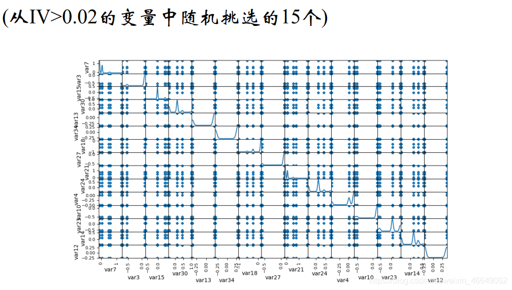
corrCols = random.sample(WOE_encoding, 15)
sampleDf = trainData[corrCols]
# 将列名重命名
for col in corrCols:
    sampleDf.rename(columns={
    
    col: col_to_index[col]}, inplace=True)
# 画散布矩阵图
scatter_matrix(sampleDf, alpha=0.2, figsize=(6, 6), diagonal='kde')

# 多因子分析
# 如果变量两两之间存在高度相关性，则选择具有较高IV的变量
# 迭代器
compare = list(combinations(varByIV, 2))
removed_var = []
roh_thresould = 0.5
for pair in compare:
    (x1, x2) = pair
    # 返回皮尔逊相关系数
    roh = np.corrcoef([trainData[str(x1) + "_WOE"], trainData[str(x2) + "_WOE"]])[0, 1]
    if abs(roh) >= roh_thresould:
        if var_IV[x1] > var_IV[x2]:
            removed_var.append(x2)
            del trainData[x2]
        else:
            removed_var.append(x1)
            del trainData[x1]

# 检验多变量之间的共线性—起变量挑选作用，也可以在模型构建中使用l1正则化，达到同样的效果
selected_by_corr = [i for i in varByIV if i not in removed_var]
for i in range(len(selected_by_corr)):
    x0 = trainData[selected_by_corr[i] + '_WOE']
    x0 = np.array(x0)
    X_Col = [k + '_WOE' for k in selected_by_corr if k != selected_by_corr[i]]
    X = trainData[X_Col]
    X = np.matrix(X)
    regr = LinearRegression()
    clr = regr.fit(X, x0)
    x_pred = clr.predict(X)
    R2 = 1 - ((x_pred - x0.mean()) ** 2).sum() / ((x0 - x0.mean()) ** 2).sum()
    vif = 1 / (1 - R2)
    if vif > 10:
        print("warning : the vif for {0} is {1}".format(selected_by_corr[i], vif))
trainData.to_csv('data/allData_2.csv', header=True, encoding='gbk', columns=allData.columns, index=False)