线性回归
在统计学中,线性回归是对标量响应和一个或多个解释变量(也称为因变量和自变量)之间关系建模的一种线性方法。
近年来,线性线性回归在人工智能和机器学习领域发挥了重要作用。线性回归算法因其相对简单和众所周知的特性而成为监督机器学习的基本算法之一。感兴趣的读者可以参考深度学习方面的资料,例如Andrew Ng从深度学习的角度很好地介绍了线性回归(到第7页)。
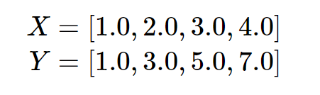
但是,由于这不是一门深度学习的课程,所以我们将从数学的角度来解决这个问题。我们从学习一个具体的例子开始,给出以下数据(在深度学习的术语中,这些数据被称为训练数据):
我们的目标是生成一个线性函数:![]()
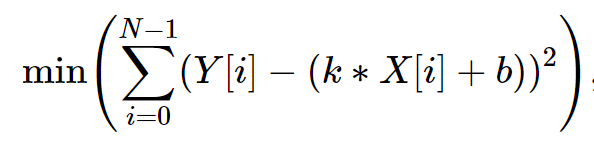
使其拟合上述数据尽可能接近,其中变量和为未知变量。通过“尽可能接近”,我们使用最小二乘法,即我们要最小化以下表达式:
 N 是X 或Y 的长度
现在下一步是解方程(6)来计算变量的值和。我们将使用Z3来完成这个任务,因为Z3也支持一些非线性约束求解。
Exercise 18:阅读linear_regression.py Python文件中的代码,您需要安装matplotlib包来运行这段代码。你可以通过pip安装matplotlib:
pip install matplotlib或者,你可以通过PyChram的偏好安装它们,就像我们在作业1的软件设置中所做的那样。在设置环境之后,完成lr_training()方法,使用Z3进行线性回归。
import matplotlib.pyplot as plt
from z3 import *
from linear_regression_ml import sklearn_lr
class Todo(Exception):
def __init__(self, msg):
self.msg = msg
def __str__(self):
return self.msg
def __repr__(self):
return self.__str__()
################################################
# Linear Regression (from the SMT point of view)
# In statistics, linear regression is a linear approach to modelling
# the relationship between a scalar response and one or more explanatory
# variables (also known as dependent and independent variables).
# The case of one explanatory variable is called simple linear regression;
# for more than one, the process is called multiple linear regression.
# This term is distinct from multivariate linear regression, where multiple
# correlated dependent variables are predicted, rather than a single scalar variable.
# In recent years, linear Linear regression plays an important role in the
# field of artificial intelligence such as machine learning. The linear
# regression algorithm is one of the fundamental supervised machine-learning
# algorithms due to its relative simplicity and well-known properties.
# Interested readers can refer to the materials on deep learning,
# for instance, Andrew Ng gives a good introduction to linear regression
# from a deep learning point of view.
# However, as this is not a deep learning course, so we'll concentrate
# on the mathematical facet. And you should learn the background
# knowledge on linear regression by yourself.
# We start by studying one concrete example, given the following data
# (in machine learning terminology, these are called the training data):
xs = [1.0, 2.0, 3.0, 4.0]
ys = [1.0, 3.0, 5.0, 7.0]
# our goal is to produce a linear function:
# y = k*x + b
# such that it fits the above data as close as possible, where
# the variables "k" and "b" are unknown variables.
# By "as close as possible", we use a least square method, that is, we
# want to minimize the following expression:
# min(\sum_i (ys[i] - (k*xs[i]+b)^2) (1)
# Now the next step is to solve the equation (1) to calculate the values
# for the variables "k" and "b".
# The popular approach used extensively in deep learning is the
# gradient decedent algorithm, if you're interested in this algorithm,
# here is a good introduction from Andrew Ng (up to page 7):
# https://see.stanford.edu/materials/aimlcs229/cs229-notes1.pdf
# In the following, we'll discuss how to solve this problem using
# SMT technique from this course.
# Both "draw_points()" and "draw_line()" are drawing utility functions to
# draw points and straight line.
# You don't need to understand these code, and you can skip
# these two functions safely. If you are really interested,
# please refer to the manuals of matplotlib library.
# Input: xs and ys are the given data for the coordinates
# Output: draw these points [xs, ys], no explicit return values.
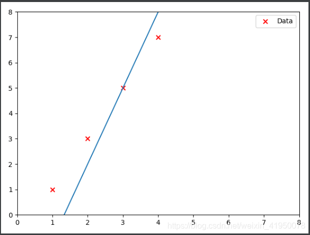
def draw_points(xs, ys):
plt.scatter(xs, ys, marker='x', color='red', s=40, label='Data')
plt.legend(loc='best')
plt.xlim(0, 8) # 设定绘图范围
plt.ylim(0, 8)
plt.savefig("./points.png")
plt.show()
# Input: a group of coordinates [xs, ys]
# k and b are coefficients
# Output: draw the coordinates [xs, ys], draw the line y=k*x+b
# no explicit return values
def draw_line(k, b, xs, ys):
new_ys = [(k*xs[i]+b) for i in range(len(xs))]
plt.scatter(xs, ys, marker='x', color='red', s=40, label='Data')
plt.plot(xs, new_ys)
plt.legend(loc='best')
plt.xlim(0, 8) # 设定绘图范围
plt.ylim(0, 8)
plt.savefig("./line.png")
plt.show()
# Arguments: xs, ys, the given data for these coordinates
# Return:
# 1. the solver checking result "res";
# 2. the k, if any;
# 3. the b, if any.
def lr_training(xs, ys):
# create two coefficients
k, b = Ints('k b')
# exercise 18: Use a least squares method
# (https://en.wikipedia.org/wiki/Least_squares)
# to generate the target expression which will be minimized
# Your code here:
# raise Todo("exercise 18: please fill in the missing code.")
exps = []
i = 0
for x in xs:
exps.append((ys[i] - k*x - b)*(ys[i] - k*x - b))
i = i+1
# print(exps)
# double check the expression is right,
# it should output:
#
# 0 +
# (1 - k*1 - b)*(1 - k*1 - b) +
# (3 - k*2 - b)*(3 - k*2 - b) +
# (5 - k*3 - b)*(5 - k*3 - b) +
# (7 - k*4 - b)*(7 - k*4 - b)
#
print("the target expression is: ")
print(sum(exps))
# create a solver
solver = Optimize()
# add some constraints into the solver, these are the feasible values
solver.add([k < 100, k > 0, b > -10, b < 10])
# tell the solver which expression to check
solver.minimize(sum(exps))
# kick the solver to perform checking
res = solver.check()
# return the result, if any
if res == sat:
model = solver.model()
kv = model[k]
bv = model[b]
return res, kv.as_long(), bv.as_long()
else:
return res, None, None
if __name__ == '__main__':
draw_points(xs, ys)
res, k, b = lr_training(xs, ys)
if res == sat:
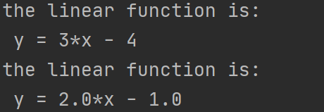
print(f"the linear function is:\n y = {k}*x {'+' if b >= 0 else '-'} {abs(b)}")
draw_line(k, b, xs, ys)
else:
print('\033[91m Training failed! \033[0m')
k, b = sklearn_lr(xs, ys)
print(f"the linear function is:\n y = {k}*x {'+' if b >= 0 else '-'} {abs(b)}")
# exercise 19: Compare the machine learning approach and the LP approach
# by trying some different training data. Do the two algorithms produce the same
# results? What conclusion you can draw from the result?
# Your code here:
输出结果:
深度学习中广泛使用的流行方法是gradient decedent算法,如果你对这个算法感兴趣,上面Andrew Ng的笔记中包含了很好的介绍。在大多数情况下,你不需要重新发明轮子,Python中有很多有效的机器学习库,比如scikit-learn。您可以直接使用它们来完成任务。
Exercise 19:在linear_regression_ml.py Python文件中,我们提供了一个基于scikit-learn深度学习库的线性回归实现。你不需要写任何代码,但你需要通过pip安装numpy和scikit-learn包:
pip install numpy
pip install scikit-learn
或者,你可以通过PyChram的偏好安装它们,就像我们在作业1的软件设置中所做的那样。设置环境之后,您需要比较机器学习方法和LP方法(您在练习17中通过尝试一些不同的训练数据实现的方法)。这两种算法产生相同的结果吗?从结果中你能得出什么结论?
此题有疑问、下周更。= =
#中科大软院-hbj形式化课程笔记-欢迎留言与私信交流
#随手点赞,我会更开心~~^_^