利用线性回归实现鸢尾花数据集分类

从鸢尾花数据集中挑选山鸢尾(iris-Setosa)和变色鸢尾(iris-Versicolor) 两种花的信息作为测试数据。出于可视化的原因，只考虑数据集中萼片长度(sepla length)和花瓣长度(petal length)这两个特征。

import pandas as pd
df = pd.read_csv(r'http://archive.ics.uci.edu/ml/machine-learning-databases/iris/iris.data')
df.tail()

	5.1	3.5	1.4	0.2	Iris-setosa
144	6.7	3.0	5.2	2.3	Iris-virginica
145	6.3	2.5	5.0	1.9	Iris-virginica
146	6.5	3.0	5.2	2.0	Iris-virginica
147	6.2	3.4	5.4	2.3	Iris-virginica
148	5.9	3.0	5.1	1.8	Iris-virginica

y = df.iloc[0:99, 4].values
y

array(['Iris-setosa', 'Iris-setosa', 'Iris-setosa', 'Iris-setosa',
       'Iris-setosa', 'Iris-setosa', 'Iris-setosa', 'Iris-setosa',
       'Iris-setosa', 'Iris-setosa', 'Iris-setosa', 'Iris-setosa',
       'Iris-setosa', 'Iris-setosa', 'Iris-setosa', 'Iris-setosa',
       'Iris-setosa', 'Iris-setosa', 'Iris-setosa', 'Iris-setosa',
       'Iris-setosa', 'Iris-setosa', 'Iris-setosa', 'Iris-setosa',
       'Iris-setosa', 'Iris-setosa', 'Iris-setosa', 'Iris-setosa',
       'Iris-setosa', 'Iris-setosa', 'Iris-setosa', 'Iris-setosa',
       'Iris-setosa', 'Iris-setosa', 'Iris-setosa', 'Iris-setosa',
       'Iris-setosa', 'Iris-setosa', 'Iris-setosa', 'Iris-setosa',
       'Iris-setosa', 'Iris-setosa', 'Iris-setosa', 'Iris-setosa',
       'Iris-setosa', 'Iris-setosa', 'Iris-setosa', 'Iris-setosa',
       'Iris-setosa', 'Iris-versicolor', 'Iris-versicolor',
       'Iris-versicolor', 'Iris-versicolor', 'Iris-versicolor',
       'Iris-versicolor', 'Iris-versicolor', 'Iris-versicolor',
       'Iris-versicolor', 'Iris-versicolor', 'Iris-versicolor',
       'Iris-versicolor', 'Iris-versicolor', 'Iris-versicolor',
       'Iris-versicolor', 'Iris-versicolor', 'Iris-versicolor',
       'Iris-versicolor', 'Iris-versicolor', 'Iris-versicolor',
       'Iris-versicolor', 'Iris-versicolor', 'Iris-versicolor',
       'Iris-versicolor', 'Iris-versicolor', 'Iris-versicolor',
       'Iris-versicolor', 'Iris-versicolor', 'Iris-versicolor',
       'Iris-versicolor', 'Iris-versicolor', 'Iris-versicolor',
       'Iris-versicolor', 'Iris-versicolor', 'Iris-versicolor',
       'Iris-versicolor', 'Iris-versicolor', 'Iris-versicolor',
       'Iris-versicolor', 'Iris-versicolor', 'Iris-versicolor',
       'Iris-versicolor', 'Iris-versicolor', 'Iris-versicolor',
       'Iris-versicolor', 'Iris-versicolor', 'Iris-versicolor',
       'Iris-versicolor', 'Iris-versicolor', 'Iris-versicolor'],
      dtype=object)

import numpy as np
import matplotlib.pyplot as plt
y = np.where(y == 'Iris-setosa', -1, 1)
x = df.iloc[0: 99, [0, 2]].values
plt.scatter(x[:49, 0], x[:49, 1], color='red', marker='o', label='setosa')
plt.scatter(x[49:99, 0], x[49: 99, 1], color='blue', marker='x', label='versicolor')
plt.xlabel('petal length')
plt.ylabel('sepal length')
plt.legend(loc='upper left')
plt.show()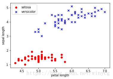

这里需要定义出一条线性回归线用于分类，需要再图中定义分类的线性函数：
权值向量为$w= \begin{bmatrix} w_{0}\\ w_{1}\\ w_{2} \end{bmatrix}$,$x= \begin{bmatrix} 1\\ x_{1}\\ x_{2} \end{bmatrix}$

$$z=w_{0}+x_{1}w_{1}+x_{2}w_{2}=w^{T}x$$
标签判定函数：
$$\phi (z)=\left\{\begin{matrix} 1, z\geq 0 \\ -1, z<0 \end{matrix}\right.$$

误差函数：

$$J(w)=\frac{1}{2n}\sum_{i}(y^{i}-z^{i})^{2}$$
求解偏导数：
$$\frac{\partial{J(w)}}{\partial w_{j}}=\frac{1}{2n}\sum_{i}2(y^{i}-z^{i})\frac{\partial (y^{i}-z^{i})}{w_{j}}=-\frac{1}{n}\sum_{i}(y^{i}-z^{i})x^{i}_{j}$$
更新权重：
$$w_{j}:=w_{j}-\eta \frac{\partial{J(w)}}{\partial w_{j}},j=0,1,2$$
采用批量梯度下降进行优化：

import numpy as np  
import pandas as pd  
import matplotlib.pyplot as plt  
from matplotlib.colors import ListedColormap  


class AdalineBGD:  
    def __init__(self, eta=0.01, n_iter=50):  
        self.eta = eta  
        self.n_iter = n_iter  

    def fit(self, X, y):  
        self.w_ = np.zeros(X.shape[1]+1)  
        self.J_ = []  

        for _ in range(self.n_iter):  
            z = np.dot(X, self.w_[1:]) + self.w_[0]  
            self.w_[0] += self.eta * (y - z).sum()
            self.w_[1:] += self.eta * np.dot(X.T, (y - z))  
            self.J_.append(((y-z)**2).sum()*0.5)  
        return self  

    def predict(self, X):  
        return np.where(np.dot(X, self.w_[1:]) + self.w_[0] >= 0.0, 1, -1)  


def plot_decision_regions(X, y, classifier, ax):  

    # setup marker generator and color map  
    markers = ('o', 'x')  
    colors = ('blue', 'red')  
    cmap = ListedColormap(colors[:len(np.unique(y))])  

    # plot the decision region  
    x1_min, x1_max = X[:, 0].min() - 1, X[:, 0].max() + 1  
    x2_min, x2_max = X[:, 1].min() - 1, X[:, 1].max() + 1  
    xx1, xx2 = np.meshgrid(np.arange(x1_min, x1_max, 0.02), np.arange(x2_min, x2_max, 0.02))  
    z = classifier.predict(np.array([xx1.flatten(), xx2.flatten()]).T)  
    z = z.reshape(xx1.shape)  
    plt.contourf(xx1, xx2, z, cmap=cmap, alpha=0.3)  
    plt.xlim(x1_min, x1_max)  
    plt.ylim(x2_min, x2_max)  

    # plot class samples  
    for idx, cl in enumerate(np.unique(y)):  
        ax[1].scatter(x=X[y == cl, 0], y=X[y == cl, 1], cmap=cmap(idx), marker=markers[idx], label=cl, alpha=1)
    ax[1].legend(loc='best')
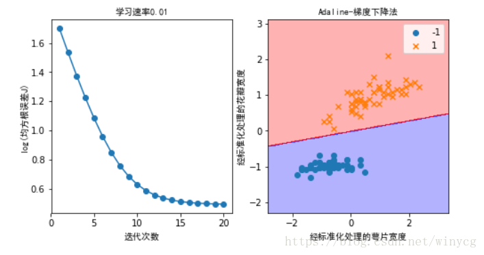
    ax[1].set_title('Adaline-梯度下降法', fontproperties='SimHei')  
    ax[1].set_xlabel('经标准化处理的萼片宽度', fontproperties='SimHei')  
    ax[1].set_ylabel('经标准化处理的花瓣宽度', fontproperties='SimHei')  


df = pd.read_csv(r'http://archive.ics.uci.edu/ml/machine-learning-databases/iris/iris.data')  
y = df.iloc[:100, 4].values  
y = np.where(y == 'Iris-setosa', -1, 1)  
X = df.iloc[:100, [0, 2]].values  
X_std = X.copy()  
X_std[:, 0] = (X[:, 0] - X[:, 0].mean()) / X[:, 0].std()  
X_std[:, 1] = (X[:, 1] - X[:, 1].mean()) / X[:, 1].std()  


fig1, ax1 = plt.subplots(1, 2, figsize=(8, 4))  
demo = AdalineBGD(n_iter=20, eta=0.01).fit(X_std, y)  
plot_decision_regions(X_std, y, demo, ax1)  
ax1[0].plot(range(1, len(demo.J_)+1), np.log10(demo.J_), marker='o')  
ax1[0].set_title('学习速率0.01', fontproperties='SimHei')  
ax1[0].set_xlabel('迭代次数', fontproperties='SimHei')  
ax1[0].set_ylabel('log(均方根误差J)', fontproperties='SimHei')  


plt.show()