目录
熟悉Jupyter环境下的python编程,在Jupyter下完成一个鸢尾花数据集的线性多分类、可视化显示与测试精度实验。
支持向量机&鸢尾花Iris数据集的SVM线性分类练习.
一、鸢尾花数据集分类
1、萼片
获取数据集
import numpy as np
from sklearn.linear_model import LogisticRegression
import matplotlib.pyplot as plt
import matplotlib as mpl
from sklearn import datasets
from sklearn import preprocessing
import pandas as pd
from sklearn.preprocessing import StandardScaler
from sklearn.pipeline import Pipeline
df = pd.read_csv('http://archive.ics.uci.edu/ml/machine-learning-databases/iris/iris.data', header=0)
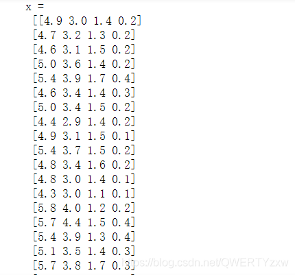
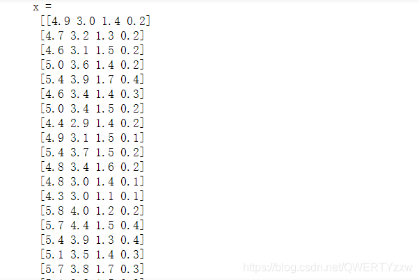
x = df.values[:, :-1]
y = df.values[:, -1]
print('x = \n', x)
print('y = \n', y)
le = preprocessing.LabelEncoder()
le.fit(['Iris-setosa', 'Iris-versicolor', 'Iris-virginica'])
print(le.classes_)
y = le.transform(y)
print('Last Version, y = \n', y)
数据处理
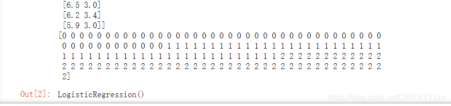
x = x[:, :2]
print(x)
print(y)
x = StandardScaler().fit_transform(x)
lr = LogisticRegression()   # Logistic回归模型
lr.fit(x, y.ravel())        # 根据数据[x,y],计算回归参数
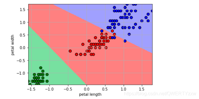
绘制分类图样
N, M = 500, 500 # 横纵各采样多少个值
x1_min, x1_max = x[:, 0].min(), x[:, 0].max() # 第0列的范围
x2_min, x2_max = x[:, 1].min(), x[:, 1].max() # 第1列的范围
t1 = np.linspace(x1_min, x1_max, N)
t2 = np.linspace(x2_min, x2_max, M)
x1, x2 = np.meshgrid(t1, t2) # 生成网格采样点
x_test = np.stack((x1.flat, x2.flat), axis=1) # 测试点
cm_light = mpl.colors.ListedColormap(['#77E0A0', '#FF8080', '#A0A0FF'])
cm_dark = mpl.colors.ListedColormap(['g', 'r', 'b'])
y_hat = lr.predict(x_test) # 预测值
y_hat = y_hat.reshape(x1.shape) # 使之与输入的形状相同
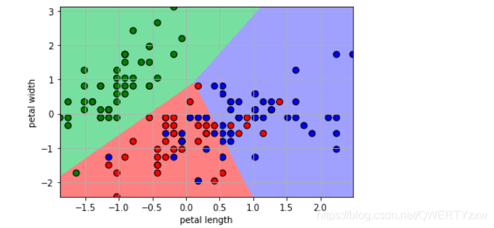
plt.pcolormesh(x1, x2, y_hat, cmap=cm_light) # 预测值的显示
plt.scatter(x[:, 0], x[:, 1], c=y.ravel(), edgecolors='k', s=50, cmap=cm_dark)
plt.xlabel('petal length')
plt.ylabel('petal width')
plt.xlim(x1_min, x1_max)
plt.ylim(x2_min, x2_max)
plt.grid()
plt.show()
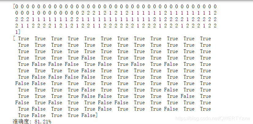
模型预测
y_hat = lr.predict(x)
y = y.reshape(-1)
result = y_hat == y
print(y_hat)
print(result)
acc = np.mean(result)
print('准确度: %.2f%%' % (100 * acc))
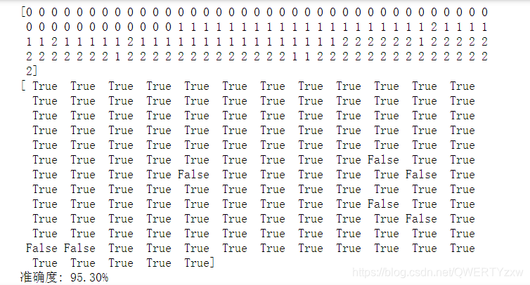
2、花瓣
import numpy as np
from sklearn.linear_model import LogisticRegression
import matplotlib.pyplot as plt
import matplotlib as mpl
from sklearn import datasets
from sklearn import preprocessing
import pandas as pd
from sklearn.preprocessing import StandardScaler
from sklearn.pipeline import Pipeline
df = pd.read_csv('http://archive.ics.uci.edu/ml/machine-learning-databases/iris/iris.data', header=0)
x = df.values[:, :-1]
y = df.values[:, -1]
print('x = \n', x)
print('y = \n', y)
le = preprocessing.LabelEncoder()
le.fit(['Iris-setosa', 'Iris-versicolor', 'Iris-virginica'])
print(le.classes_)
y = le.transform(y)
print('Last Version, y = \n', y)
x = x[:, 2:]
print(x)
print(y)
x = StandardScaler().fit_transform(x)
lr = LogisticRegression()   # Logistic回归模型
lr.fit(x, y.ravel())        # 根据数据[x,y],计算回归参数
N, M = 500, 500     # 横纵各采样多少个值
x1_min, x1_max = x[:, 0].min(), x[:, 0].max()   # 第0列的范围
x2_min, x2_max = x[:, 1].min(), x[:, 1].max()   # 第1列的范围
t1 = np.linspace(x1_min, x1_max, N)
t2 = np.linspace(x2_min, x2_max, M)
x1, x2 = np.meshgrid(t1, t2)                    # 生成网格采样点
x_test = np.stack((x1.flat, x2.flat), axis=1)   # 测试点

cm_light = mpl.colors.ListedColormap(['#77E0A0', '#FF8080', '#A0A0FF'])
cm_dark = mpl.colors.ListedColormap(['g', 'r', 'b'])
y_hat = lr.predict(x_test)       # 预测值
y_hat = y_hat.reshape(x1.shape)                 # 使之与输入的形状相同
plt.pcolormesh(x1, x2, y_hat, cmap=cm_light)     # 预测值的显示
plt.scatter(x[:, 0], x[:, 1], c=y.ravel(), edgecolors='k', s=50, cmap=cm_dark)
plt.xlabel('petal length')
plt.ylabel('petal width')
plt.xlim(x1_min, x1_max)
plt.ylim(x2_min, x2_max)
plt.grid()
plt.show()
y_hat = lr.predict(x)
y = y.reshape(-1)
result = y_hat == y
print(y_hat)
print(result)
acc = np.mean(result)
print('准确度: %.2f%%' % (100 * acc))
二、总结与参考资料
1、总结
Python对数据的分析方面有很大的便捷。