决策树
决策树(Decision Tree)是一种基本的分类与回归方法,当决策树用于分类时称为分类树,用于回归时称为回归树。主要介绍分类树。
决策树由结点和有向边组成。结点有两种类型:内部结点和叶结点,其中内部结点表示一个特征或属性,叶结点表示一个类。
决策树学算法通常是一个递归地选择最优特征,并根据该特征对训练数据进行分割,使得对各个子数据集有一个最好的分类的过程。根据信息增益准则的特征选择方法:对于训练数据集(或子集),计算其每个特征的信息增益,并比较它们的大小,选择信息增益最大的特征。
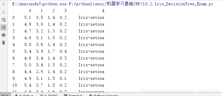
数据集
代码
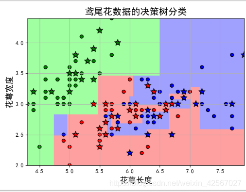
不同深度情况下的分类
// An highlighted block
import numpy as np
import pandas as pd
import matplotlib.pyplot as plt
import matplotlib as mpl
from sklearn.tree import DecisionTreeClassifier
from sklearn.model_selection import train_test_split
# 花萼长度、花萼宽度,花瓣长度,花瓣宽度
iris_feature_E = 'sepal length', 'sepal width', 'petal length', 'petal width'
iris_feature = u'花萼长度', u'花萼宽度', u'花瓣长度', u'花瓣宽度'
iris_class = 'Iris-setosa', 'Iris-versicolor', 'Iris-virginica'
if __name__ == "__main__":
mpl.rcParams['font.sans-serif'] = [u'SimHei']
mpl.rcParams['axes.unicode_minus'] = False
'''加载数据'''
data = pd.read_csv('F:\pythonlianxi\shuju\iris.data', header=None)
#print(data)
#样本集
x = data[range(4)]
#标签集
y = pd.Categorical(data[4]).codes
# 为了可视化,仅使用前两列特征
x = x.iloc[:, :2]
#样本集,标签集分为测试集和验证集
x_train, x_test, y_train, y_test = train_test_split(x, y, train_size=0.7, random_state=1)
#print(y_test.shape)
print('开始训练模型....')
#
'''决策树'''
# 决策树参数估计
# min_samples_split = 10:如果该结点包含的样本数目大于10,则(有可能)对其分支
# min_samples_leaf = 10:若将某结点分支后,得到的每个子结点样本数目都大于10,则完成分支;否则,不进行分支
#建立决策树模型
model = DecisionTreeClassifier(criterion='entropy')
model.fit(x_train, y_train)
#测试数据
y_test_hat = model.predict(x_test) # 测试数据
# 横纵各采样值
N, M = 50, 50
x1_min, x2_min = x.min()
x1_max, x2_max = x.max()
t1 = np.linspace(x1_min, x1_max, N)
t2 = np.linspace(x2_min, x2_max, M)
# 生成网格采样点
x1, x2 = np.meshgrid(t1, t2)
# 测试点
x_show = np.stack((x1.flat, x2.flat), axis=1)
#图形颜色
cm_light = mpl.colors.ListedColormap(['#A0FFA0', '#FFA0A0', '#A0A0FF'])
cm_dark = mpl.colors.ListedColormap(['g', 'r', 'b'])
# 预测值
y_show_hat = model.predict(x_show)
# 使之与输入的形状相同
y_show_hat = y_show_hat.reshape(x1.shape)
# print (y_show_hat)
'''绘图'''
plt.figure(facecolor='w')
plt.pcolormesh(x1, x2, y_show_hat, cmap=cm_light) # 预测值的显示
plt.scatter(x_test[0], x_test[1], c=y_test.ravel(), edgecolors='k', s=150, zorder=10, cmap=cm_dark, marker='*') # 测试数据
plt.scatter(x[0], x[1], c=y.ravel(), edgecolors='k', s=40, cmap=cm_dark) # 全部数据
plt.xlabel(iris_feature[0], fontsize=15)
plt.ylabel(iris_feature[1], fontsize=15)
plt.xlim(x1_min, x1_max)
plt.ylim(x2_min, x2_max)
plt.grid(True)
plt.title(u'鸢尾花数据的决策树分类', fontsize=17)
plt.show()
#
'''测试样本'''
# 训练集上的预测结果
y_test = y_test.reshape(-1)
print( y_test_hat)
print (y_test)
result = (y_test_hat == y_test) # True则预测正确,False则预测错误
#取平均
acc = np.mean(result)
print('准确度: %.2f%%' % (100 * acc))
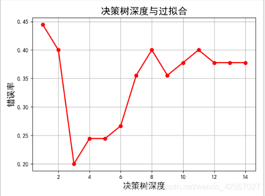
'''过拟合'''
# 过拟合:错误率
#给定深度14层
depth = np.arange(1, 15)
err_list = []
#每个深度进行测试
for d in depth:
clf = DecisionTreeClassifier(criterion='entropy', max_depth=d)
clf.fit(x_train, y_train)
y_test_hat = clf.predict(x_test) # 测试数据
result = (y_test_hat == y_test) # True则预测正确,False则预测错误
if d == 1:
print (result)
err = 1 - np.mean(result)
err_list.append(err)
print (d, ' 错误率: %.2f%%' % (100 * err))
'''绘图'''
plt.figure(facecolor='w')
plt.plot(depth, err_list, 'ro-', lw=2)
plt.xlabel(u'决策树深度', fontsize=15)
plt.ylabel(u'错误率', fontsize=15)
plt.title(u'决策树深度与过拟合', fontsize=17)
plt.grid(True)
plt.show()
实验分析
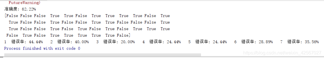
准确度: 62.22%,决策树深度为3时可以达到较高的识别率。