文章目录
数据集
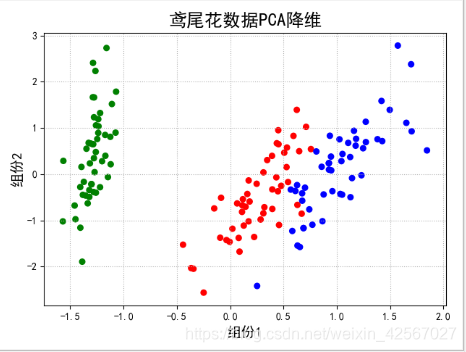
鸢尾花数据集有三个类别,每个类别有50个样本。其中一个类别与另外两个线性可分,另外两个不能线性可分。
代码实现
PCA降维原理和使用python和matlab实现降维
https://blog.csdn.net/weixin_42567027/article/details/107418146
PCA降维
最好先了解PCA原理,这样PCA后的数据就好理解了。
// An highlighted block
import pandas as pd
import numpy as np
from sklearn.decomposition import PCA
from sklearn.linear_model import LogisticRegressionCV
from sklearn import metrics
from sklearn.model_selection import train_test_split
import matplotlib as mpl
import matplotlib.pyplot as plt
import matplotlib.patches as mpatches
from sklearn.pipeline import Pipeline
from sklearn.preprocessing import PolynomialFeatures

def extend(a, b):
    return 1.05*a-0.05*b, 1.05*b-0.05*a

if __name__ == '__main__':
    pd.set_option('display.width', 200)

    '''加载数据'''
    data = pd.read_csv('F:\pythonlianxi\iris.csv', header=None)
    #设置列标签
    columns = ['sepal_length', 'sepal_width', 'petal_length', 'petal_width', 'type']
    #rename:用于命名文件或目录
    data.rename(columns=dict(zip(np.arange(5), columns)), inplace=True)
    #Categorical:将类别信息转化成数值信息,因此将type中的数据类型进行转化
    data['type'] = pd.Categorical(data['type']).codes
    #print (data)
    '''数据集和标签集'''
    #x存储的是除type类外的数据,也就是数据集
    x = data.loc[:, columns[:-1]]
    #y中存储的是type数据,也就是标签集
    y = data['type']
    #print(x)

    '''pca降维'''
    #输出的方差  可以结合pca降维的原理来理解
    #n_components:组分的个数选择,在这个算法中,选择的是前两个组分
    pca = PCA(n_components=2, whiten=True, random_state=0)
    #利用PCA降维技术对数据进行某种统一处理(比如标准化~N(0,1),将数据缩放(映射)到某个固定区间,归一化,正则化等)
    x = pca.fit_transform(x)
    #pca之后,前两个组分在所有数据中所占信息的比例,一般来说80%的比例,说明已经具有较大的代表性。
    print( '各方向方差:', pca.explained_variance_)
    print ('方差所占比例:', pca.explained_variance_ratio_)
  #  print (x[:5])

    '''绘图'''
    #颜色选择
    cm_light = mpl.colors.ListedColormap(['#77E0A0', '#FF8080', '#A0A0FF'])
    cm_dark = mpl.colors.ListedColormap(['g', 'r', 'b'])
    #文字转化
    mpl.rcParams['font.sans-serif'] = u'SimHei'
    mpl.rcParams['axes.unicode_minus'] = False
    # #绘图
    plt.figure(facecolor='w')
    plt.scatter(x[:, 0], x[:, 1], s=30, c=y, marker='o', cmap=cm_dark)
    #print(x[:, 0])
    plt.grid(b=True, ls=':')
    #打标签  fontsize:字体大小
    plt.xlabel(u'组份1', fontsize=14)
    plt.ylabel(u'组份2', fontsize=14)
    plt.title(u'鸢尾花数据PCA降维', fontsize=18)
    plt.show()
logistic回归分析
// An highlighted block
'''使用逻辑回归模型进行分类识别'''
#训练集和测试集按 7:3分开
x, x_test, y, y_test = train_test_split(x, y, train_size=0.7)
#训练模型
model = Pipeline([
#PolynomialFeatures:特征选择 degree:选择线性函数次数
('poly', PolynomialFeatures(degree=3, include_bias=True)),
('lr', LogisticRegressionCV(Cs=np.logspace(-3, 4, 8), cv=5, fit_intercept=False))])
#调参
model.fit(x, y)
print ('最优参数:', model.get_params('lr')['lr'].C_)
#使用生成的模型进行分类识别
y_hat = model.predict(x)
print('训练集精确度:', metrics.accuracy_score(y, y_hat))
y_test_hat = model.predict(x_test)
print('测试集精确度:', metrics.accuracy_score(y_test, y_test_hat))
'''绘图'''
#对得到的结果进行绘图,即在PCA的图形上根据分类结果对不同类别进行绘制
N, M = 500, 500 # 横纵各采样多少个值
# x得到的数据的第0列的范围
x1_min, x1_max = extend(x[:, 0].min(), x[:, 0].max())
# x得到的数据的第1列的范围
x2_min, x2_max = extend(x[:, 1].min(), x[:, 1].max())
t1 = np.linspace(x1_min, x1_max, N)
t2 = np.linspace(x2_min, x2_max, M)
# 生成网格采样点
x1, x2 = np.meshgrid(t1, t2)
# 测试点
x_show = np.stack((x1.flat, x2.flat), axis=1)
# 预测值
y_hat = model.predict(x_show)
# 使之与输入的形状相同
y_hat = y_hat.reshape(x1.shape)
plt.figure(facecolor='w')
plt.pcolormesh(x1, x2, y_hat, cmap=cm_light) # 预测值的显示
plt.scatter(x[:, 0], x[:, 1], s=30, c=y, edgecolors='k', cmap=cm_dark) # 样本的显示
#打标签
plt.xlabel(u'组份1', fontsize=14)
plt.ylabel(u'组份2', fontsize=14)
#对x,y坐标轴的坐标进行限制
plt.xlim(x1_min, x1_max)
plt.ylim(x2_min, x2_max)
plt.grid(b=True, ls=':')
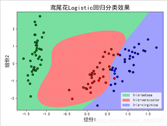
patchs = [mpatches.Patch(color='#77E0A0', label='Iris-setosa'),
mpatches.Patch(color='#FF8080', label='Iris-versicolor'),
mpatches.Patch(color='#A0A0FF', label='Iris-virginica')]
plt.legend(handles=patchs, fancybox=True, framealpha=0.8, loc='lower right')
plt.title(u'鸢尾花Logistic回归分类效果', fontsize=17)
plt.show()

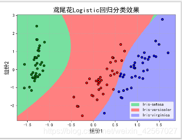
模型泛化能力分析
由于做线性回归预测时候,为了提高模型的泛化能力,经常采用多次线性函数建立模型。次数越多,学习的内容越多,但是也容易造成过拟合。
当使用二次函数时,即degree=2
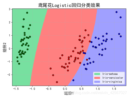
当使用三次函数时,即degree=3
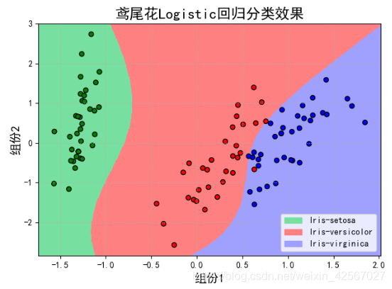
当使用四次函数时,即degree=4
对这个数据集的LR分类+模型评估
https://blog.csdn.net/weixin_42567027/article/details/107423666