1 项目描述
使用逻辑回归算法来对鸢尾花进行分类;
数据集包括训练数据train.txt和测试数据test.txt;测试数据中,每个样本包括特定的几个特征参数,最后是一个类别标签,而测试数据中的样本则只包括了特征参数
2 逻辑回归:鸢尾花数据集分类
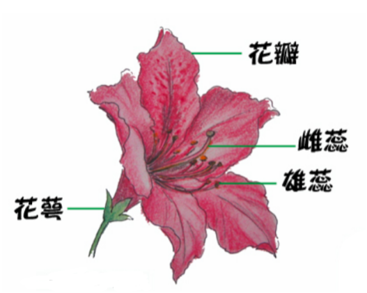
2.1 鸢尾花数据信息
-
Sepal length: 花萼长度
-
Sepal width: 花萼宽度
-
Petal length: 花瓣长度
-
Petal width: 花瓣宽度
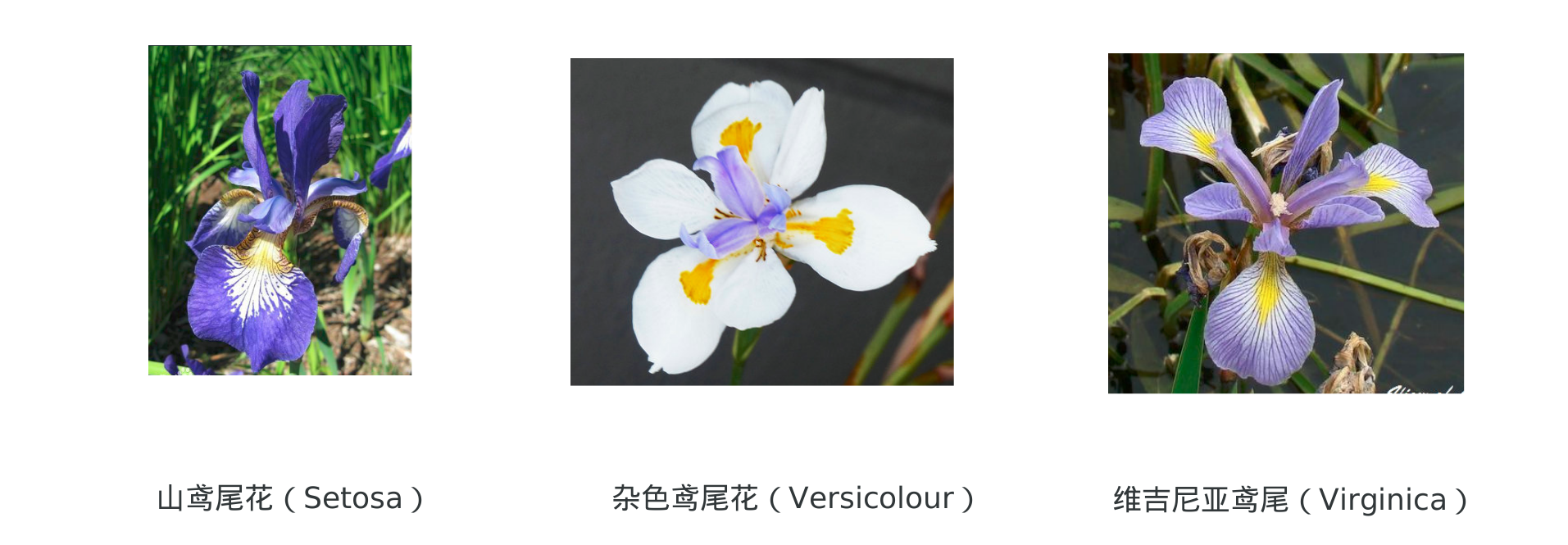
2.2 鸢尾花分类
2.3 问题描述
如果: 花萼长度,花萼宽度, 花瓣长度,花瓣宽度为5.1, 3.5, 1.4, 0.2
问:是什么花
3 分析问题
3.1 加载数据集
def load_data():
    """
    加载数据集
    :return:
        X: 花瓣宽度
        Y: 鸢尾花类型
    """
    # 加载sklearn包自带的鸢尾花数据;
    iris = datasets.load_iris()
    # # 查看鸢尾花的数据集
    # print(iris)
    # # 查看鸢尾花的key值;
    # # dict_keys(['data', 'target', 'target_names', 'DESCR','feature_names', 'filename'])
    # print(iris.keys())
    # # 获取鸢尾花的特性: ['sepal length (cm)', 'sepal width (cm)', 'petal length (cm)', 'petal width (cm)']
    # print(iris['feature_names'])
    # print(iris['data'])
    # print(iris['target'])
    # 因为花瓣的相关系数比较高, 所以分类效果比较好, 所以我们就用花瓣宽度当作x;
    X = iris['data'][:, 3:]
    # 获取分类的结果
    Y = iris['target']
    return  X, Y
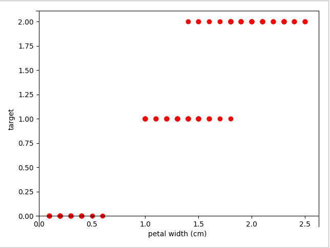
3.2 可视化展示
图形配置
def configure_plt(plt):
    """
    配置图形的坐标表信息
    """
    # 获取当前的坐标轴, gca = get current axis
    ax = plt.gca()
    # 设置x轴, y周在(0, 0)的位置
    ax.spines['bottom'].set_position(('data', 0))
    ax.spines['left'].set_position(('data', 0))

    # 绘制x,y轴说明
    plt.xlabel('petal width (cm)')  # 花瓣宽度
    plt.ylabel('target')    # 鸢尾花类型
    return  plt
- 绘图
def draw_pic():
    X, Y = load_data()
    import  matplotlib.pyplot as plt
    import matplotlib.pyplot as plt
    plt.scatter(X,  Y,   c='red')
    plt = configure_plt(plt)

    # 显示图
    plt.show()


if __name__ == '__main__':
    draw_pic()
3.4 训练模型
def model_train():
    """
    训练模型
    :return:
    """
    # 通过上面的数据做逻辑回归
    """
    multi_class='ovr' : 分类方式; OvR(One vs Rest),一对剩余的意思,有时候也称它为  OvA(One vs All);一般使用 OvR,更标准;
    solver='sag',逻辑回归损失函数的优化方法;  sag:即随机平均梯度下降,是梯度下降法的变种
    """
    log_reg = LogisticRegression(multi_class='ovr', solver='sag')
    X, Y = load_data()
    log_reg.fit(X, Y)
    print('w0:', log_reg.coef_)
    print('w1:', log_reg.intercept_)
    return  log_reg
3.5 数据集预测及可视化
def test_data(log_reg):
    """
    测试数据集
    :param log_reg:
    :return:
    """
    # 创建新的数据集去测试
    #   np.linespace 用于创建等差数列的函数, 会创建一个从0到3的等差数列, 包含1000个值;
    #   reshape生成1000行1列的数组;
    X_new = np.linspace(0, 3, 1000).reshape(-1, 1)
    # print(X_new)
    y_proba = log_reg.predict_log_proba(X_new)
    y_hat = log_reg.predict(X_new)
    print(y_proba)
    print(y_hat)
    return  X_new, y_hat

def draw_pic():
    """
    绘制图形
    :return:
    """
    X, Y = load_data()
    log_reg = model_train()
    test_X, test_Y = test_data(log_reg)
    import matplotlib.pyplot as plt
    plt.scatter(X,  Y,   c='red')
    plt.scatter(test_X,  test_Y,   c='green')
    plt = configure_plt(plt)

    # 显示图
    plt.show()


if __name__ == '__main__':
    draw_pic()
3.6 完整源代码
"""
文件名: 01_iris_classification.py
创建时间: 2019-04-20 11:
作者: lvah
联系方式: [email protected]
代码描述:


逻辑回归(处理鸢尾花数据集)

"""

import numpy as np
from sklearn import datasets
from sklearn.linear_model import LogisticRegression


def load_data():
    """
    加载数据集
    :return:
        X: 花瓣宽度
        Y: 鸢尾花类型
    """
    # 加载sklearn包自带的鸢尾花数据;
    iris = datasets.load_iris()
    # # 查看鸢尾花的数据集
    # print(iris)
    # # 查看鸢尾花的key值;
    # # dict_keys(['data', 'target', 'target_names', 'DESCR','feature_names', 'filename'])
    # print(iris.keys())
    # # 获取鸢尾花的特性: ['sepal length (cm)', 'sepal width (cm)', 'petal length (cm)', 'petal width (cm)']
    # print(iris['feature_names'])
    # print(iris['data'])
    # print(iris['target'])
    # 因为花瓣的相关系数比较高, 所以分类效果比较好, 所以我们就用花瓣宽度当作x;
    X = iris['data'][:, 3:]
    # 获取分类的结果
    Y = iris['target']
    return  X, Y


def configure_plt(plt):
    """
    配置图形的坐标表信息
    """
    # 获取当前的坐标轴, gca = get current axis
    ax = plt.gca()
    # 设置x轴, y周在(0, 0)的位置
    ax.spines['bottom'].set_position(('data', 0))
    ax.spines['left'].set_position(('data', 0))

    # 绘制x,y轴说明
    plt.xlabel('petal width (cm)')  # 花瓣宽度
    plt.ylabel('target')    # 鸢尾花类型
    return  plt


def model_train():
    """
    训练模型
    :return:
    """
    # 通过上面的数据做逻辑回归
    """
    multi_class='ovr' : 分类方式; OvR(One vs Rest),一对剩余的意思,有时候也称它为  OvA(One vs All);一般使用 OvR,更标准;
    solver='sag',逻辑回归损失函数的优化方法;  sag:即随机平均梯度下降,是梯度下降法的变种
    """
    log_reg = LogisticRegression(multi_class='ovr', solver='sag')
    X, Y = load_data()
    log_reg.fit(X, Y)
    print('w0:', log_reg.coef_)
    print('w1:', log_reg.intercept_)
    return  log_reg


def test_data(log_reg):
    """
    测试数据集
    :param log_reg:
    :return:
    """
    # 创建新的数据集去测试
    #   np.linespace 用于创建等差数列的函数, 会创建一个从0到3的等差数列, 包含1000个值;
    #   reshape生成1000行1列的数组;
    X_new = np.linspace(0, 3, 1000).reshape(-1, 1)
    # print(X_new)
    y_proba = log_reg.predict_log_proba(X_new)
    y_hat = log_reg.predict(X_new)
    print(y_proba)
    print(y_hat)
    return  X_new, y_hat

def draw_pic():
    """
    绘制图形
    :return:
    """
    X, Y = load_data()
    log_reg = model_train()
    test_X, test_Y = test_data(log_reg)
    import matplotlib.pyplot as plt
    plt.scatter(X,  Y,   c='red')
    plt.scatter(test_X,  test_Y,   c='green')
    plt = configure_plt(plt)

    # 显示图
    plt.show()


if __name__ == '__main__':
    draw_pic()
4 问题解决方案
import numpy as np
from sklearn import datasets
from sklearn.linear_model import  LogisticRegression


iris = datasets.load_iris()
X = iris['data']
Y = iris['target']

log_reg = LogisticRegression(multi_class='ovr', solver='sag', max_iter=10000)
log_reg.fit(X, Y)


X_new = [[5.1, 3.5, 1.4, 0.2]]
print(log_reg.predict_proba(X_new))
print(log_reg.predict(X_new))
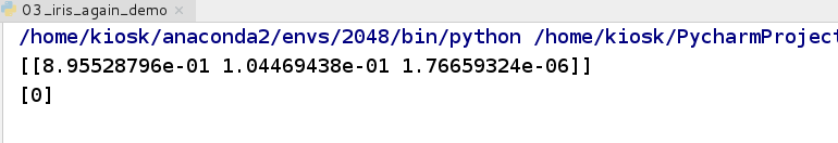
- 预测鸢尾花的类型为山鸢尾花.