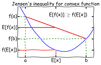
EM (Expectation–Maximization) Algorithm 思路分析及推导

往期文章链接目录

Jensen’s inequality

• Theorem: Let $f$ be a convex function, and let $X$ be a random variable. Then:

$E[f(X)] \geq f(E[X])$

$\quad$ Moreover, if $f$ is strictly convex, then $E[f(X)] = f(E[X])$ holds true if and
only if $X$ is a constant.

• Later in the post we are going to use the following fact from the Jensen’s inequality:
  Suppose $\lambda_j \geq 0$ for all $j$ and $\sum_j \lambda_j = 1$, then

$\log \sum_j \lambda_j y_j \geq \sum_j \lambda_j \, log \, y_j$

$\quad$ where the $\log$ function is concave.

Overview of Expectation–Maximization (EM) algorithm

In this post, let $Y$ be a set of observed data, $Z$ a set of unobserved latent data, and $\theta$ the unknown parameters.

(After this post, you will be comfortable with the following description about the EM algorithm.)

Expectation–Maximization (EM) algorithm is an iterative method to find (local) maximum likelihood estimation (MLE) of $L(\theta) = p(Y|\theta)$, where the model depends on unobserved latent variables $Z$.

Algorithm:

1. Initialize peremeters $\theta_0$.

Iterate between steps 2 and 3 until convergence:

2. an expectation (E) step, which creates a function $Q(\theta, \theta_i)$ for the expectation of the log-likelihood $\log p(Y,Z|\theta)$ evaluated using the current conditional distribution of
   $Z$ given $Y$ and the current estimate of the parameters $\theta_i$, where

$\begin{aligned} Q(\theta, \theta_i) &= \sum_Z P(Z|Y,\theta_i) \cdot \log p(Y,Z|\theta) \\ &= E_{Z \sim P(Z|Y,\theta_i)}[\log p(Y,Z|\theta)] \end{aligned}$

3. A maximization (M) step, which computes parameters maximizing the expected log-likelihood $Q(\theta, \theta_i)$ found on the $E$ step and then update parameters to $\theta_{i+1}$.

These parameter-estimates are then used to determine the distribution of the latent variables in the next $E$ step. We say it converges if the increase in successive iterations is smaller than some tolerance parameter.

In general, multiple maxima may occur, with no guarantee that the global maximum will be found.

Intuition: Why we need EM algorithm

Sometimes maximizing the likelihood $\ell(\theta)$ explicitly might be difficult since there are some unknown latent variables. In such a setting, the EM algorithm gives an efficient method for maximum likelihood estimation.

Complete Case v.s. Incomplete Case

Complete case

$(Y, Z)$ is observable, and the log likelihood can be written as

$\begin{aligned} \ell(\theta) &= \log p(Y, Z | \theta) \\ &= \log p(Z|\theta) \cdot p(Y|Z, \theta) \\ &= \log p(Z|\theta) + \log p(Y|Z, \theta) \\ \end{aligned}$

We subdivide our task of maximizing $\ell(\theta)$ into two sub-tasks. Note that in both $\log p(Z|\theta)$ and $\log p(Y|Z, \theta)$, the only unknown parameter is $\theta$. They are just two standard MLE problems which could be easily solved by methods such as gradient descent.

Incomplete case

$(Y)$ is observable, but $(Z)$ is unknown. We need to introduce the marginal distribution of variable $Z$:

$\begin{aligned} \ell(\theta) &= \log p(Y | \theta) \\ &= \log \sum_Z p(Y, Z | \theta) \\ &= \log \sum_Z p(Z|\theta) \cdot p(Y|Z, \theta) \\ \end{aligned}$

Here we have a summation inside the log, so it’s hard to use optimization methods or take derivatives. This is the case where EM algorithm comes into aid.

EM Algorithm Derivation (Using MLE)

Given the observed data $Y$, we want to maximize the likelihood $\ell(\theta) = p(Y|\theta)$, and it’s the same as maximizing the log-likelihood $\log p(Y|\theta)$. Therefore, from now on we will try to maximize the likelihood

$\ell(\theta) = \log p(Y|\theta)$

by taking the unknown variable $Z$ into account, we rewrite the objective function as

$\begin{aligned} \ell(\theta) &= \log p(Y|\theta) \\ &= \log \sum_Z p(Y, Z | \theta) \\ &= \log \sum_Z p(Y|Z,\theta) \cdot p(Z|\theta) \\ \end{aligned}$

Note that in the last step, the $\log$ is outside of the $\sum$, which is hard to compute and optimize. Check out my previous post to know why we prefer to have $\log$ inside of $\sum$, instead of outside. So later we would find a way to approximate it (Jensen’s inequality).

Suppose we follow the iteration step 2 (E) and 3 (M) repeatedly, and have updated parameters to $\theta_i$, then the difference between $\ell(\theta)$ and our estimate $\ell(\theta_i)$ is $\ell(\theta) - \ell(\theta_i)$. You can think of this difference as the improvement that later estimate of $\theta$ tries to achieve. So our next step is to find $\theta_{i+1}$ such that it improves the difference the most. That is, to make the difference $\ell(\theta) - \ell(\theta_i)$ as large as possible. So we want our next estimate $\theta_{i+1}$ to be

$\theta_{i+1} = \mathop{\rm arg\,max}\limits_{\theta} \,\, \ell(\theta) - \ell(\theta_i)$

Note that we know the value of $\theta_i$, so as $\ell(\theta_i)$. And

$\begin{aligned} \ell(\theta) - \ell(\theta_i)&= \log p(Y|\theta) \\ &= \log \sum_Z p(Y|Z,\theta) \cdot p(Z|\theta) - \log p(Y|\theta_i) \\ &= \log \sum_Z P(Z|Y,\theta_i) \frac{p(Y|Z,\theta) \cdot p(Z|\theta)}{P(Z|Y,\theta_i)} - \log p(Y|\theta_i) & & &(1)\\ \end{aligned}$

Since $P(Z|Y,\theta_i) \geq 0$ for all $z\in Z$ and $\sum_Z P(Z|Y,\theta_i) = 1$, we can use the Jensen’s inequality and then re-write $(1)$ as

$\begin{aligned} \ell(\theta) - \ell(\theta_i) &\geq \sum_Z P(Z|Y,\theta_i) \log \frac{p(Y|Z,\theta) \cdot p(Z|\theta)}{P(Z|Y,\theta_i)} - \sum_Z P(Z|Y,\theta_i)) \cdot \log p(Y|\theta_i)\\ &= \sum_Z P(Z|Y,\theta_i) \left( \log \frac{p(Y|Z,\theta) \cdot p(Z|\theta)}{P(Z|Y,\theta_i)} - \log p(Y|\theta_i) \right) \\ \ell(\theta) &\geq \ell(\theta_i) + \sum_Z P(Z|Y,\theta_i) \log \frac{p(Y|Z,\theta) \cdot p(Z|\theta)}{P(Z|Y,\theta_i) \cdot p(Y|\theta_i)} \end{aligned}$

Now we define

$B(\theta, \theta_i) \triangleq \ell(\theta_i) + \sum_Z P(Z|Y,\theta_i) \log \frac{p(Y|Z,\theta) \cdot p(Z|\theta)}{P(Z|Y,\theta_i) \cdot p(Y|\theta_i)}$

So we see that

$\ell(\theta) \geq B(\theta, \theta_i)$

which implies that $B(\theta, \theta_i)$ is a lower bound of $\ell(\theta)$ for all $i$. Therefore our next step is to maximize the lower bound $B(\theta, \theta_i)$ and make it as tight as possible. In the $M$ step, we define

$\begin{aligned} \theta_{i+1} &= \mathop{\rm arg\,max}\limits_{\theta} B(\theta, \theta_i)\\ &= \mathop{\rm arg\,max}\limits_{\theta} \, \left(\ell(\theta_i) + \sum_Z P(Z|Y,\theta_i) \cdot \log \frac{p(Y|Z,\theta) \cdot p(Z|\theta)}{P(Z|Y,\theta_i) \cdot p(Y|\theta_i)} \right) && (2)\\ &= \mathop{\rm arg\,max}\limits_{\theta} \, \left(\sum_Z P(Z|Y,\theta_i) \cdot \log \frac{p(Y|Z,\theta) \cdot p(Z|\theta)}{P(Z|Y,\theta_i) \cdot p(Y|\theta_i)} \right) && (3)\\ &= \mathop{\rm arg\,max}\limits_{\theta} \, \left(\sum_Z P(Z|Y,\theta_i) \cdot [\log p(Y|Z,\theta) \cdot p(Z|\theta) - \log P(Z|Y,\theta_i) \cdot p(Y|\theta_i)] \right) && (4)\\ &= \mathop{\rm arg\,max}\limits_{\theta} \, \left(\sum_Z P(Z|Y,\theta_i) \cdot \log p(Y|Z,\theta) \cdot p(Z|\theta) \right) && (5)\\ &= \mathop{\rm arg\,max}\limits_{\theta} \, \left(\sum_Z P(Z|Y,\theta_i) \cdot \log p(Y,Z|\theta) \right) &&(6)\\ &= \mathop{\rm arg\,max}\limits_{\theta} \, Q(\theta, \theta_i) &&(7)\\ \end{aligned}$

Remark:

• $(2) \to (3)$ since $\ell(\theta_i)$ does not contain $\theta$.

• $(3) \to (4)$ we used $\log \frac{A}{B} = \log A - \log B$.

• $(4) \to (5)$ since $\log P(Z|Y,\theta_i) \cdot p(Y|\theta_i)$ does not contain $\theta$.

• $(6) \to (7)$ we define $Q(\theta, \theta_i) = \sum_Z P(Z|Y,\theta_i) \cdot \log p(Y,Z|\theta)$.

• since both $Y$ and $\theta_i$ are known, we have the distribution of $Z \sim p(Z|Y,\theta_i)$. Therefore, the only unknown parameter is $\theta$, which means this is now a complete case I mentioned early in the post. So this is now a MLE problem.

summary

1. $\theta_{i+1} = \mathop{\rm arg\,max}\limits_{\theta} \ell(\theta) - \ell(\theta_i) = \mathop{\rm arg\,max}\limits_{\theta} \, Q(\theta, \theta_i)$. This implies that maximizing $\ell(\theta) - \ell(\theta_i)$ is the same as maximizing $Q(\theta, \theta_i)$.

2. Note that $Q(\theta, \theta_i) = \sum_Z P(Z|Y,\theta_i) \cdot \log p(Y,Z|\theta)$ is just the expectation of $\log p(Y,Z|\theta)$, where $Z$ is drawn from the current conditional distribution $P(Z|Y,\theta_i)$. Therefore we have
   $Q(\theta, \theta_i) = E_{Z \sim p(Z|Y,\theta_i)}[\log p(Y,Z|\theta)]$
   That’s why it’s called the Expectation step. In E step, we are actually trying to calculate the expectation of the term $\log p(Y,Z|\theta)$, where unknown variable $Z$ follows the current conditional distribution given by $Y$ and $\theta_i$. Then in the Maximazation step, we are trying to maximize this expectation. That’s why it’s called the M step.

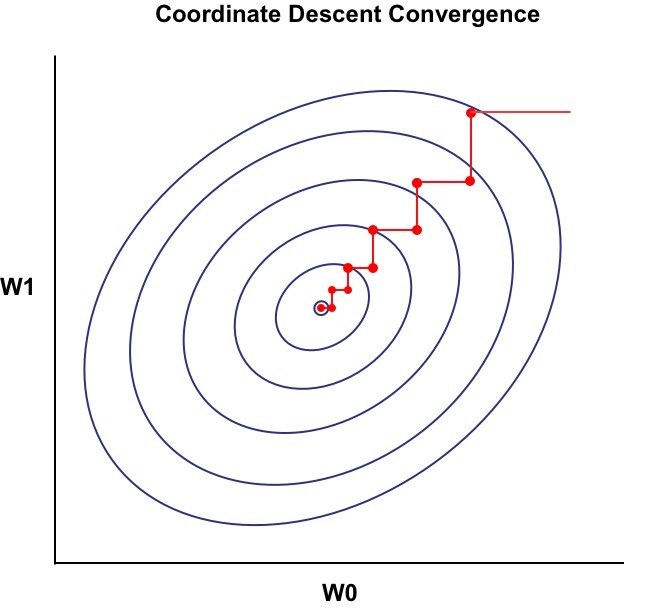
Coordinate Ascent/ descent - view EM from a different prospect

In the Expectation Step, we actually fixed $\theta_i$, and tried to optimize $Q(\theta, \theta_i)$.

In the Maximization step, we actually fixed $Q(\theta, \theta_i)$, and tried to optimize $\theta$ to get $\theta_{i+1}$.

Every time we only optimize one variable and fix the rest. Therefore, from the graph above we see that in every iteration the gradient changes either vertically or horizontally.

To see how to perform the coordinate descent, check out my previous post.

Convergence of EM algorithm

By following the algorithm, we keep updating parameter $\theta_i$ and calculating approximated log-likelihood $\ell (\theta_i)$. But do we actually keep $\ell (\theta_i)$ getting closer to $l(\theta)$ as we do more iterations? Keep in mind that in MLE our final goal is to maximize $\ell (\theta)$.

Suppose $\theta_i$ and $\theta_{i+1}$ are the parameters from two successive iterations of EM. We will now prove that $\ell(\theta_i) \leq \ell(\theta_{i+1})$, which shows EM always monotonically improves the log-likelihood.

$\begin{aligned} \ell(\theta) &= \log p(Y|\theta) \\ &= \log \frac {p(Y,Z|\theta)}{p(Z|Y, \theta)} \\ &= \log p(Y,Z|\theta) - \log p(Z|Y, \theta) \\ &= \sum_Z p(Z|Y, \theta_i)\cdot \log p(Y,Z|\theta) - \sum_Z p(Z|Y, \theta_i)\cdot \log p(Z|Y, \theta) \\ &= Q(\theta, \theta_i) + H(\theta, \theta_i) && (8)\\ \end{aligned}$

where $H(\theta, \theta_i) = - \sum_Z p(Z|Y, \theta_i)\cdot \log p(Z|Y, \theta)$. This last equation $(8)$ holds for every value of $\theta$, including $\theta=\theta_i$, which means

$\ell(\theta_i) = Q(\theta_i, \theta_i) + H(\theta_i, \theta_i)$

Therefore subtracting $\ell(\theta_i)$ from $\ell(\theta_{i+1})$ gives

$\begin{aligned} \ell(\theta_{i+1}) - \ell(\theta_i) &= [Q(\theta_{i+1}, \theta_{i}) + H(\theta_{i+1}, \theta_{i})] - [Q(\theta_i, \theta_i) + H(\theta_i, \theta_i)]\\ &= [Q(\theta_{i+1}, \theta_{i}) - Q(\theta_i, \theta_{i})] + [H(\theta_{i+1}, \theta_{i}) - H(\theta_i, \theta_{i})] \\ \end{aligned}$

Since $\theta_{i+1} = \mathop{\rm arg\,max}\limits_{\theta} \, Q(\theta, \theta_i)$, we have $Q(\theta_{i+1}, \theta_i) \geq Q(\theta_i, \theta_i)$. The second parenthesis gives

$\begin{aligned} H(\theta_{i+1}, \theta_{i}) - H(\theta_i, \theta_{i}) &= - \sum_Z p(Z|Y, \theta_i)\cdot \log p(Z|Y, \theta_{i+1}) + \sum_Z p(Z|Y, \theta_i)\cdot \log p(Z|Y, \theta_i) \\ &= - \left( \sum_Z p(Z|Y, \theta_i)\cdot \log p(Z|Y, \theta_{i+1}) - \sum_Z p(Z|Y, \theta_i)\cdot \log p(Z|Y, \theta_i)\right) \\ &= - \left( \sum_Z p(Z|Y, \theta_i) \cdot \log \frac{p(Z|Y, \theta_{i+1})}{p(Z|Y, \theta_{i})} \right) && \,\,\,(9)\\ &\geq - \log \left( \sum_Z p(Z|Y, \theta_i) \cdot \frac{p(Z|Y, \theta_{i+1})}{p(Z|Y, \theta_{i})} \right) && (10)\\ &= - \log \sum_Z p(Z|Y, \theta_{i+1}) = - \log 1 = 0 \end{aligned}$

From $(9)$ to $(10)$ we use the Jensen’s inequality (note that there is a negative sign in the front so we reverse the inequality).

Since $Q(\theta_{i+1}, \theta_{i}) \geq Q(\theta_i, \theta_{i})$ and $H(\theta_{i+1}, \theta_{i}) \geq H(\theta_i, \theta_{i})$, we have

$\ell(\theta_{i+1}) \geq \ell(\theta_i) \qquad\qquad \text{for all} \, i$

Since it’s monotonically increasing and bounded above, we say $\ell (\theta_i)$ converges.

What’s next?

I’m going to write a post to discuss how EM algorithm is applied in K-means and GMM in the future. Stay tuned!

---

Reference:

• https://en.wikipedia.org/wiki/Expectation–maximization_algorithm
• Part IX: The EM algorithm from CS229 Lecture notes by Andrew Ng http://cs229.stanford.edu/notes/cs229-notes8.pdf
• http://guillefix.me/cosmos/static/Jensen%27s%2520inequality.html
• https://en.wikipedia.org/wiki/Jensen%27s_inequality
• http://www.adeveloperdiary.com/data-science/machine-learning/introduction-to-coordinate-descent-using-least-squares-regression/

往期文章链接目录