吴恩达机器学习python代码练习一（线性回归）

吴恩达机器学习练习文件下载地址：
链接：https://pan.baidu.com/s/1RvUeG10FBpV9RyFtOX1Zdw
提取码：5b4x

单变量线性回归

import numpy as np
import matplotlib.pyplot as plt

path = 'E:\吴恩达\作业代码资料\全部作业代码-无答案\ML_totalexerise\exerise1\ex1data1.txt'
data = np.loadtxt(path,delimiter=',')#delimiter为分隔符
x_data = np.array(data)[:,0]
y_data = np.array(data)[:,1]

数据可视化

plt.scatter(x_data,y_data)
plt.xlabel('population')
plt.ylabel('profit')

假设函数：

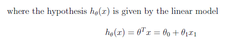
#定义假设函数
def hypoth(theta,x):
    return x.dot(theta)

代价函数：

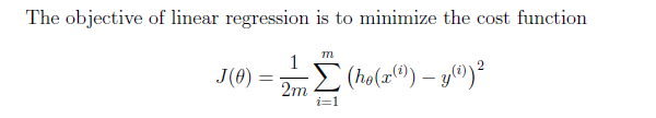
#定义代价函数
def costFunction(theta,x,y):
    return np.sum(np.power(hypoth(theta,x)-y,2))/(2*len(y))

批量梯度下降函数：

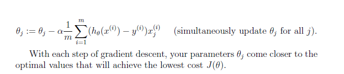
#定义批量梯度下降函数
def bgd(theta,x,y,alpha):
    second = (alpha/len(y))*(x.T.dot(hypoth(theta,x)-y))
    return theta - second

#初始化各项参数
#np.insert中文教程地址：http://codingdict.com/article/21577
x_array = np.insert(x_data.reshape(len(y_data),1),0,1,axis=1)#输入数组、索引、插入的数值、插入的轴（0-行，1-列）
theta = np.zeros(x_array.shape[1])
alpha = 0.01 #学习速率
iterations = 1500 #迭代步数

运行下代价函数，若初始值为32.07，那么代价函数运行正常

costFunction(theta,x_array,y_data)

32.072733877455676

loss = np.zeros(iterations)
for iteration in range(iterations):
    cost = costFunction(theta,x_array,y_data)
    theta = bgd(theta,x_array,y_data,alpha)
    loss[iteration] = cost

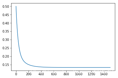
#查看代价函数随迭代步数的变化趋势，一直减小计算正确
plt.plot(range(iterations),loss)

#求得的theta1和theta2
theta

array([-3.63029144,  1.16636235])

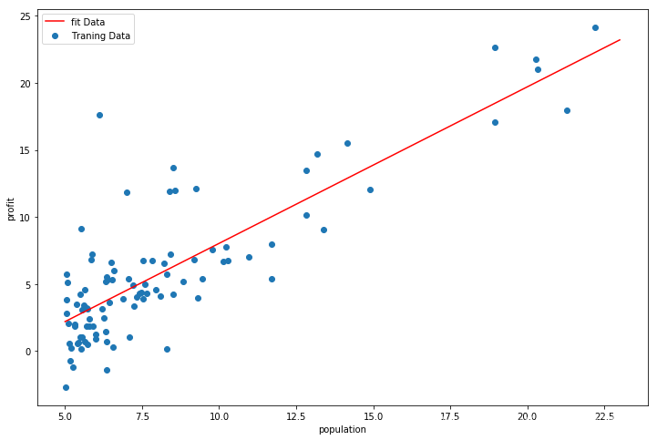
def fit(theta,x):
    return theta[0] +theta[1]*x

fig,ax = plt.subplots(figsize=(12,8))
ax.scatter(x_data,y_data,label='Traning Data')
x = np.linspace(5,23,100)
ax.plot(x,fit(theta,x),'r',label='fit Data')
ax.legend()
plt.xlabel('population')
plt.ylabel('profit')

多变量线性回归

path2 = 'E:\吴恩达\作业代码资料\全部作业代码-无答案\ML_totalexerise\exerise1\ex1data2.txt'
data2 = np.loadtxt(path2,delimiter=',')#delimiter为分隔符

#数据预处理
data2_array = np.array(data2)
x2_data = data2_array[:,0:-1]
y2 = data2_array[:,-1]

#由于多变量存在数据之间相差较大的情况，因此需要对其进行归一化，使算法更快收敛
#x_min = x_data.max(axis = 0)# 可以指定关键字参数axis来获得行最大（小）值或列最大（小）值
# axis=0 行方向最大（小）值，即获得每列的最大（小）值
# axis=1 列方向最大（小）值，即获得每行的最大（小）值
#返回的是位置（索引）
#print(a.argmax(axis=0)) #[1 2 1 2]
x2_data_gui = (x2_data-x2_data.mean(axis = 0))/x2_data.std(axis = 0 )
x2_array = np.insert(x2_data_gui,0,1,axis=1)
y2_array = (y2-y2.mean(axis = 0))/y2.std(axis = 0 )

theta_multi = np.zeros(x2_array.shape[1])
loss_multi = np.zeros(iterations)
for iter_multi in range(iterations):
    cost2 = costFunction(theta_multi,x2_array,y2_array)
    theta_multi = bgd(theta_multi,x2_array,y2_array,alpha)
    loss_multi[iter_multi] = cost2 

#查看代价函数随迭代步数的变化趋势，一直减小计算正确
plt.plot(range(iterations),loss_multi)