回归问题的思想(1)先找到损失函数,(2)求损失函数最小化后的参数
假设我们的数据是(m,n)有m行数据,n个特征(feature)
则我们预测函数为 :
![]()
写成向量形式为(xo=1):

ps:因为存在截距项,这里的X矩阵是n+1维的
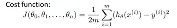
定义代价函数CostFunction:
求 minJ(θ)
得到目标函数后,我们目标是想要代价函数尽可能小,利用凸优化知识,对J(θ)求偏导并带入梯度下降公式中:
梯度下降请参考:https://www.cnblogs.com/pinard/p/5970503.html
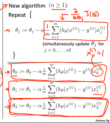
向量式:i=(1,2,...n)
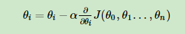
α是步长,决定更新快慢(过大可能会导致溢出)
到这里就能求出所需要的参数的更新公式。
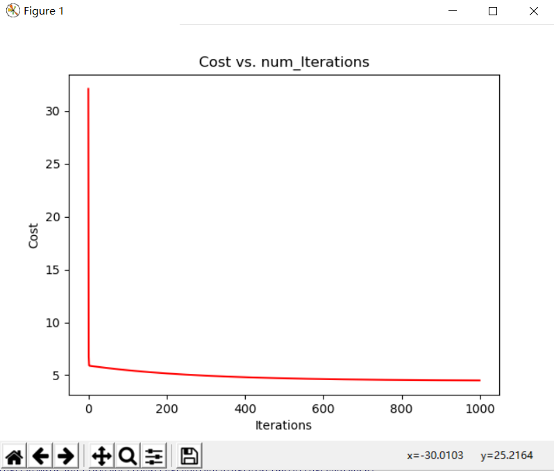
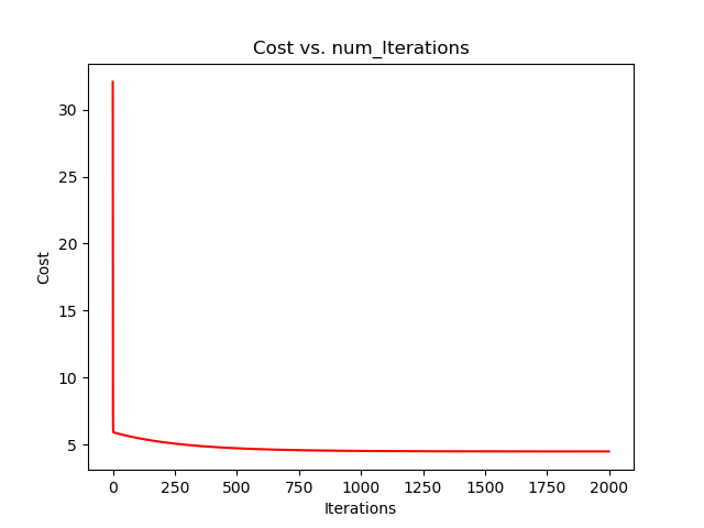
下面的例子是单变量的例子,用的随机梯度,因为可以直接画图出,比较直观。
 1 import pandas as pd
 2 import numpy as np
 3 def CostFunction(x,y,theta):
 4     med_var=np.power((x*theta)-y,2)
 5     return np.sum(med_var)/(2*len(x))
 6
 7 def Grandent(x,y,theta,alphl,maxcircle):
 8     m = x.shape[0]
 9     print('m=',m)
10     print('theta shape',theta.shape)
11     temp = np.matrix(np.zeros(theta.shape))
12     print('temp shape',temp.shape)
13     cost = np.zeros(maxcircle)  # 初始化一个ndarray,包含每次迭代的cost
14     for k in range(maxcircle):
15         # print(theta)
16         temp=theta-(alphl/m)*(x.T)*(x*theta-y)
17         cost[k]=CostFunction(x,y,theta)
18         theta=temp
19     return theta,cost
20
21
22 data=pd.read_csv('ex1data1.txt',names=['feature','price'])   #(97, 2)
23 data.insert(0,'x0',1)
24 X_dataframe=data.drop(['price'],axis=1)
25 y_dataframe=data.price
26 X=np.matrix(X_dataframe.values)  #专程矩阵格式
27 y=np.matrix(y_dataframe.values)
28 y=y.T
29 m,n=X_dataframe.shape
30 theta=np.zeros((n,1))
31 alphl=0.01  #开始设置为0.1,会一直报溢出,导致梯度下降方法不收敛
32 maxcircle=1000
33
34 theta_fin,cost=Grandent(X,y,theta,alphl,maxcircle)
35
36 import matplotlib.pyplot as plt
37
38 fig,ax = plt.subplots()
39
40 ax.plot(np.arange(maxcircle), cost, 'red')  # np.arange()返回等差数组
41 ax.set_xlabel('Iterations')
42 ax.set_ylabel('Cost')
43 ax.set_title('Cost vs. num_Iterations')
44
45 #np.linspace()在指定的间隔内返回均匀间隔的数字
46 x = np.linspace(data.feature.min(), data.feature.max(), 100) # 横坐标
47 f = theta_fin[0,0] + (theta_fin[1,0] * x)  # 纵坐标
48 fig,ax = plt.subplots()
49 ax.plot(x, f, 'r', label='Prediction')
50 ax.scatter(data['feature'], data.price, label='Traning Data')
51 ax.legend(loc=2)  # 2表示在左上角
52 ax.set_xlabel('feature')
53 ax.set_ylabel('price')
54 ax.set_title('Predicted Profit vs. Population Size')
55 plt.show()

下面是迭代1000,2000次的结果