吴恩达机器学习练习文件下载地址:
链接:https://pan.baidu.com/s/1RvUeG10FBpV9RyFtOX1Zdw
提取码:5b4x
逻辑回归(线性可分)
import pandas as pd
import numpy as np
import matplotlib.pyplot as plt
import seaborn as sns
import scipy.optimize as opt
from sklearn.metrics import classification_report#这个包是评价报告
from sklearn.preprocessing import PolynomialFeatures #特征映射
path = 'E:\吴恩达\作业代码资料\全部作业代码-无答案\ML_totalexerise\exerise2\ex2data1.txt'
# names添加列名,header用指定的行来作为标题,若原无标题且指定标题则设为None
data = pd.read_csv(path,header = None,names = ['exam1','exam2','admitted'])
# plt.figure(figsize=(10,10),dpi =160)
plt.figure(dpi =100)
sns.scatterplot('exam1','exam2',data = data,hue = 'admitted',style='admitted')

假设函数及sigmoid函数

#定义假设函数
def hyposth(theta,x):
    z = x.dot(theta)
    return 1/(1+np.exp(-z))
代价函数

#定义代价函数
def costFunction(theta,x,y):
    first = (-y)*np.log(hyposth(theta,x))
    second = (1-y)*np.log(1-hyposth(theta,x))
    return np.sum(first - second)/len(y)
梯度函数
#定义梯度函数
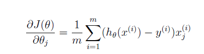
def bgd(theta, x, y):
return (x.T.dot(hyposth(theta,x)-y))/len(y)
#数据预处理
x_data = data.values[:,0:-1]
x_array = np.insert(x_data,0,1,axis=1)
y_data = data.values[:,-1]
#初始化参数
theta = np.zeros(x_array.shape[1])
costFunction(theta,x_array,y_data)
0.6931471805599453
在这里求代价函数的最小值使用scipy.optimize,计算更快。后面会使用练习一中的梯度下降函数方法进行对比。
使用opt.minimize时x0.shape必须为(n,)否则报错!!!!!!

opt.minimize官网地址:https://docs.scipy.org/doc/scipy/reference/generated/scipy.optimize.minimize.html#scipy.optimize.minimize
res = opt.minimize(fun=costFunction, x0=theta, args=(x_array, y_data), method='Newton-CG', jac=bgd)#args中为costFunction和bgd其他的参数
res
     fun: 0.20349770159353447
     jac: array([-5.22052362e-06, -1.75707267e-04, -4.65404538e-04])
 message: 'Optimization terminated successfully.'
    nfev: 72
    nhev: 0
     nit: 28
    njev: 243
  status: 0
 success: True
       x: array([-25.1614995 ,   0.20623304,   0.20147294])
使用练习一的方法中的梯度下降法求theta
#使用练习一的方法
#初始化
iterations = 10000#迭代步数
loss = np.zeros(iterations)
for iteration in range(iterations):
    cost = costFunction(theta,x_array,y_data)
    theta = theta - 0.001*bgd(theta,x_array,y_data)
    loss[iteration] = cost
plt.plot(range(iterations),loss),theta,cost

可以发现使用梯度下降法计算到10000步时,距离收敛值0.2还有很大距离,但是若将学习率0.001增大到0.01时,会导致结果震荡,因此学习率的选择非常重要!选择其他高级算法可以自动选择学习率,故使用高级优化算法是非常必要的!
对训练好的模型进行预测及验证
def predict(theta,x):
    res_pre = hyposth(theta,x)
    return [1 if x>=0.5 else 0 for x in res_pre]
y_predict = predict(res.x,x_array)
print(classification_report(y_data, y_predict))
              precision    recall  f1-score   support

         0.0       0.87      0.85      0.86        40
         1.0       0.90      0.92      0.91        60

   micro avg       0.89      0.89      0.89       100
   macro avg       0.89      0.88      0.88       100
weighted avg       0.89      0.89      0.89       100
决策边界,根据假设方程可知决策边界的方程为:
def border(theta,x):
    return -(theta[0] + theta[1]*x)/theta[-1]
x_draw = np.linspace(30,90,200)
y_draw = border(res.x,x_draw)
plt.figure(dpi =100)
sns.scatterplot('exam1','exam2',data = data,hue = 'admitted',style = 'admitted')
sns.lineplot(x_draw,y_draw)

正则化逻辑回归(非线性可分)
path2 = 'E:\吴恩达\作业代码资料\全部作业代码-无答案\ML_totalexerise\exerise2\ex2data2.txt'
data2 = pd.read_csv(path2,header = None,names = ['test1','test2','pass'])
data2.shape
(118, 3)
x2_data = data2.iloc[:,0:-1].values
y2_data = data2.iloc[:,-1].values
关于特征映射参考:
https://blog.csdn.net/AuGuSt_81/article/details/79167563?utm_source=blogxgwz8
https://www.jianshu.com/p/985884f999c1
https://blog.csdn.net/Joker_sir5/article/details/82748305?depth_1-utm_source=distribute.pc_relevant.none-task-blog-BlogCommendFromBaidu-2&utm_source=distribute.pc_relevant.none-task-blog-BlogCommendFromBaidu-2
polynomialFeatures(6)之后会返回一个新的多项式矩阵,其中第一列全为1


通过可以有更多的特征并且有更优秀的分类能力,但是也更容易出现过拟合,因此在下面我们会使用正则化来减小过拟合的出现。
#特征映射即构造多项式特征,构造之后会自动增加一列1使其与theta0相乘,不必在另外插入一列1
poly = PolynomialFeatures(6)#最高次幂
x2_data_poly = poly.fit_transform(x2_data)
x2_data_poly.shape
(118, 28)
theta_reg = np.zeros(x2_data_poly.shape[1])
lam = 1
**
正则化代价函数(注意j从1开始的,对theta0并不进行正则化)
**
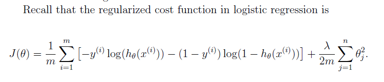
#定义正则化代价函数
def costRegfunc(theta,x,y,lam):
    theta2 = theta[1:]
    second = (lam/(2*len(y)))*np.sum(np.power(theta2,2))
    return costFunction(theta,x,y) + second
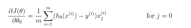
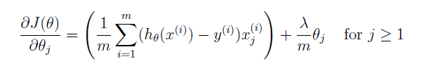
正则化梯度函数(对theta0不进行正则化 )
#正则化梯度函数
def bgdReg(theta,x,y,lam):
    reg = (lam/len(y))*theta
    reg[0] = 0
    return bgd(theta, x, y) + reg
theta_reg.shape,x2_data_poly.shape,y2_data.shape
((28,), (118, 28), (118,))
costRegfunc(theta_reg,x2_data_poly,y2_data,lam)
0.6931471805599454
res2 = opt.minimize(fun=costRegfunc, x0=theta_reg, args=(x2_data_poly, y2_data,lam), method='Newton-CG', jac=bgdReg)
res2
     fun: 0.5290027297130254
     jac: array([-2.89933074e-07, -2.97505709e-08,  9.15347119e-08, -1.76629052e-08,
        1.55193062e-08,  3.73389225e-08, -8.48293484e-09, -8.40311461e-09,
       -3.35016797e-08,  1.02909335e-07, -3.43593152e-09,  1.15039834e-09,
        1.35875173e-08,  1.23535283e-08,  2.74347823e-08, -1.23040748e-08,
       -1.05650484e-08, -1.28988259e-11,  1.10321591e-08, -1.11109068e-08,
        5.36351068e-08, -6.15402587e-09, -6.14371484e-11,  5.80157698e-09,
        4.81209604e-09,  1.10771976e-08, -3.75442831e-09,  4.67847655e-08])
 message: 'Optimization terminated successfully.'
    nfev: 7
    nhev: 0
     nit: 6
    njev: 82
  status: 0
 success: True
       x: array([ 1.27274185,  0.62527218,  1.18109103, -2.0199646 , -0.91742189,
       -1.43166715,  0.12400674, -0.36553449, -0.35723908, -0.17513158,
       -1.45815788, -0.05098904, -0.61555494, -0.2747065 , -1.19281739,
       -0.24218804, -0.20600589, -0.04473066, -0.27778463, -0.29537804,
       -0.45635817, -1.04320354,  0.0277718 , -0.29243169,  0.01556677,
       -0.32737961, -0.14388676, -0.92465329])
对训练数据进行评价
#对训练出的数据进行预测
y2_predict = predict(res2.x,x2_data_poly)
print(classification_report(y2_data, y2_predict))
              precision    recall  f1-score   support

           0       0.90      0.75      0.82        60
           1       0.78      0.91      0.84        58

   micro avg       0.83      0.83      0.83       118
   macro avg       0.84      0.83      0.83       118
weighted avg       0.84      0.83      0.83       118
绘制决策边界
x2_lins = np.linspace(-1.0, 1.0, 100)
x2_mesh, y2_mesh = np.meshgrid(x2_lins, x2_lins)
x2_ravel = x2_mesh.ravel()#转化为一维数组
x2_draw = x2_ravel.reshape(x2_ravel.shape[0],1)#转化为二维数组
y2_ravel = y2_mesh.ravel()#转化为一维数组
y2_draw = y2_ravel.reshape(y2_ravel.shape[0],1)#转化为二维数组
z_con = np.concatenate((x2_draw,y2_draw),axis = 1)#将x2_draw,y2_draw合并为一个数组进行特征映射
poly = PolynomialFeatures(6)
x2_draw_poly = poly.fit_transform(z_con)
z_draw = x2_data_poly.dot(res2.x).reshape(x2_mesh.shape)
plt.figure(dpi =100)
sns.scatterplot('test1','test2',data = data2,hue = 'pass',style= 'pass')
plt.contour(x2_mesh,y2_mesh,z_draw,0)

