1.单变量线性回归
导入包
import numpy as np
import pandas as pd
import matplotlib.pyplot as plt
导入数据集
path =  'ex1data1.txt'
data = pd.read_csv(path, header=None, names=['Population', 'Profit'])#names列名
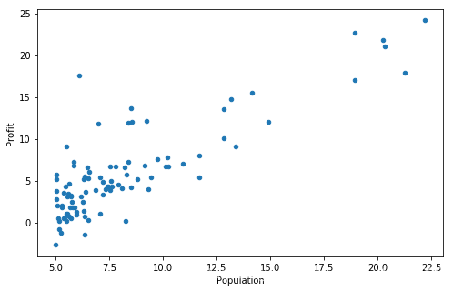
在开始任何任务之前,通过可视化来理解数据通常是有用的。
对于这个数据集,您可以使用散点图来可视化数据,因为它只有两个属性(利润和人口)。
data.plot(kind='scatter', x='Population', y='Profit', figsize=(12,8))
plt.show()
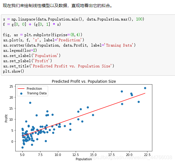
现在使用梯度下降来实现线性回归,以最小化成本函数。
首先,我们将创建一个以参数θ为特征函数的代价函数
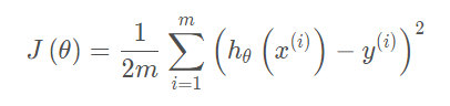
计算代价函数J(θ)
def computeCost(X, y, theta):
    # your code here  (appro ~ 2 lines)
    predictions = X*theta.T
    sqrErrors = np.square(predictions-y)
    return sum(sqrErrors)/(2*X.shape[0])
让我们在训练集中添加一列,以便我们可以使用向量化的解决方案来计算代价和梯度。
data.insert(0, 'Ones', 1)
现在我们来做一些变量初始化。
# set X (training data) and y (target variable)
cols = data.shape[1]
X = data.iloc[:,0:cols-1]#X是所有行,去掉最后一列
y = data.iloc[:,cols-1:cols]#X是所有行,最后一列
代价函数是应该是numpy矩阵,所以我们需要转换X和Y,然后才能使用它们。 我们还需要初始化theta,即把theta所有元素都设置为0.
X = np.matrix(X.values)
y = np.matrix(y.values)
# your code here  (appro ~ 1 lines)
theta = np.matrix(np.array([0,0]))     #theta 是一个(1,2)矩阵
2. batch gradient decent(批量梯度下降)
关键点在于theta0和thata1要同时更新,需要用temp进行临时存储
def gradientDescent(X, y, theta, alpha, iters):
    temp = np.matrix(np.zeros(theta.shape))   #按照theta的形状建立temp为了临时存储theta,方便进行迭代更新。
    parameters = int(theta.ravel().shape[1]) #实际就是j的个数,批量梯度中j为0和1,所以parameters为2.
    cost = np.zeros(iters)

    for i in range(iters):
        errors = X*theta.T - y  # 97-1
        for j in range(parameters):
            term = np.multiply(errors, X[:,j]) #j=1时term为errors, j=2时,X为原生X的向量值。
            temp[0,j] = theta[0,j] - alpha*(1/X.shape[0])*np.sum(term) #梯度下降公式的代码实现,将theta0和theta1存入temp

        theta = temp #更新theta,进入迭代循环
        cost[i] = computeCost(X, y, theta)

    return theta, cost

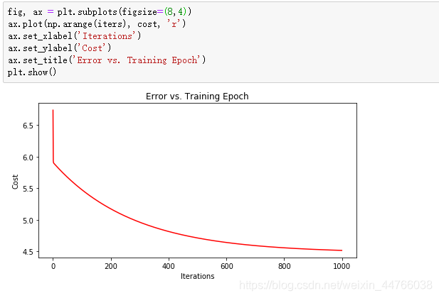
由于梯度方程式函数也在每个训练迭代中输出一个代价的向量,所以我们也可以绘制。请注意,代价总是降低 - 这是凸优化问题的一个例子。
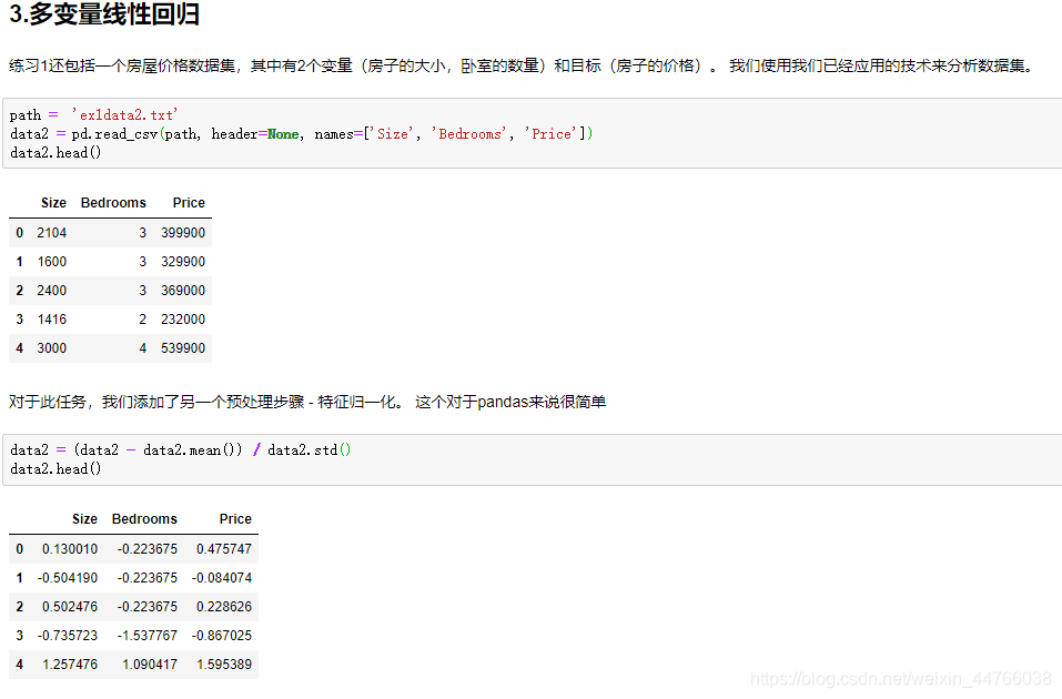
3. 多变量线性回归
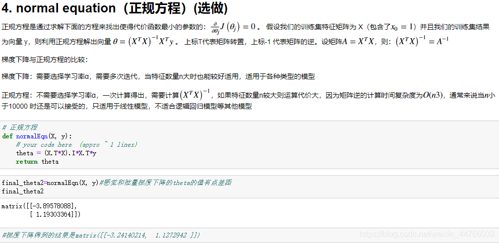
4. 正规方程
代价函数的导数等于0,求出使代价函数最小的参数(中间存在有矩阵求逆)
5. mini batch
在deep learning里面用到mini-Batch有两个原因,其中一个是因为mini-Batch会提升模型的训练速度还有一个主要原因则是,mini-batch给训练过程引入了随机性:
对于一般的BP网络来说,当没有mini-batch的时候,w、b 的每一次update都是整个数据集gradient的方向,而整个大数据集的数据分布是不会随着update的次数而改变的,它不存在随机性,这样容易是的在训练的时候 “才跑两步” cost function就卡住了,就很容易卡在saddle point或者说是local minimum 里面;如果加上mini-batch,则每次update的时候,数据集都不尽相同,都会存在一些随机性(上次update的时候是saddle point,但在下次update的时候可能就不是了),因此如果saddle point不是很麻烦的saddle point或local minimum不是很深的local minimum的话,整个模型是相对很容易跑出来的。
附录
ex1data1.txt如下:
6.1101,17.592
5.5277,9.1302
8.5186,13.662
7.0032,11.854
5.8598,6.8233
8.3829,11.886
7.4764,4.3483
8.5781,12
6.4862,6.5987
5.0546,3.8166
5.7107,3.2522
14.164,15.505
5.734,3.1551
8.4084,7.2258
5.6407,0.71618
5.3794,3.5129
6.3654,5.3048
5.1301,0.56077
6.4296,3.6518
7.0708,5.3893
6.1891,3.1386
20.27,21.767
5.4901,4.263
6.3261,5.1875
5.5649,3.0825
18.945,22.638
12.828,13.501
10.957,7.0467
13.176,14.692
22.203,24.147
5.2524,-1.22
6.5894,5.9966
9.2482,12.134
5.8918,1.8495
8.2111,6.5426
7.9334,4.5623
8.0959,4.1164
5.6063,3.3928
12.836,10.117
6.3534,5.4974
5.4069,0.55657
6.8825,3.9115
11.708,5.3854
5.7737,2.4406
7.8247,6.7318
7.0931,1.0463
5.0702,5.1337
5.8014,1.844
11.7,8.0043
5.5416,1.0179
7.5402,6.7504
5.3077,1.8396
7.4239,4.2885
7.6031,4.9981
6.3328,1.4233
6.3589,-1.4211
6.2742,2.4756
5.6397,4.6042
9.3102,3.9624
9.4536,5.4141
8.8254,5.1694
5.1793,-0.74279
21.279,17.929
14.908,12.054
18.959,17.054
7.2182,4.8852
8.2951,5.7442
10.236,7.7754
5.4994,1.0173
20.341,20.992
10.136,6.6799
7.3345,4.0259
6.0062,1.2784
7.2259,3.3411
5.0269,-2.6807
6.5479,0.29678
7.5386,3.8845
5.0365,5.7014
10.274,6.7526
5.1077,2.0576
5.7292,0.47953
5.1884,0.20421
6.3557,0.67861
9.7687,7.5435
6.5159,5.3436
8.5172,4.2415
9.1802,6.7981
6.002,0.92695
5.5204,0.152
5.0594,2.8214
5.7077,1.8451
7.6366,4.2959
5.8707,7.2029
5.3054,1.9869
8.2934,0.14454
13.394,9.0551
5.4369,0.61705
