CS231n:assignment2 SVM
一、前言
支持向量机(SVM)
kNN分类器分为两个阶段:
- 在训练过程中,分类器获取训练数据并简单地记住它;
- 在测试过程中,kNN将每个测试图像与所有的训练图像进行比较,并将k个最相似的训练图像的标签进行投票,从而决定该测试图像的类型;
具体分为两步:
①计算测试图像与训练图像每个像素点的欧氏距离
②将算得的距离进行排序,选取前k个训练图像的label,进而预测该测试图像的label - k的值是交叉验证的。
二、主要部分程序解读
1、数据处理
① 数据输入
#------------------------------svm.ipynb----------------------------------
# Load the raw CIFAR-10 data.
cifar10_dir = 'cs231n/datasets/cifar-10-batches-py'
X_train, y_train, X_test, y_test = load_CIFAR10(cifar10_dir)

# As a sanity check, we print out the size of the training and test data.
print('Training data shape: ', X_train.shape)          #Training data shape:  (50000, 32, 32, 3)
print('Training labels shape: ', y_train.shape)        #Training labels shape:  (50000,)
print('Test data shape: ', X_test.shape)			   #Test data shape:  (10000, 32, 32, 3)
print('Test labels shape: ', y_test.shape)			   #Test labels shape:  (10000,)
结果:将之前下载的cifar10_dir的数据读入进来,根据结果显示可知:
input: X_train(50000,32,32,3) y_train(50000, )
X_test(10000,32,32,3) y_test(10000, )
X_train与X_test是图片数据,而y_train和y_test则是对应图片的标签。
② 数据更新
#------------------------------svm.ipynb----------------------------------
# Split the data into train, val, and test sets. In addition we will
# create a small development set as a subset of the training data;
# we can use this for development so our code runs faster.
num_training = 49000
num_validation = 1000
num_test = 1000
num_dev = 500

# Our validation set will be num_validation points from the original training set.
mask = range(num_training, num_training + num_validation)					# 1
X_val = X_train[mask]
y_val = y_train[mask]

# Our training set will be the first num_train points from the original training set.
mask = range(num_training)													# 2
X_train = X_train[mask]
y_train = y_train[mask]

# We will also make a development set, which is a small subset of the training set.
mask = np.random.choice(num_training, num_dev, replace=False)				# 3
X_dev = X_train[mask]
y_dev = y_train[mask]

# We use the first num_test points of the original test set as our test set.
mask = range(num_test)														# 4
X_test = X_test[mask]
y_test = y_test[mask]

print('Train data shape: ', X_train.shape)				# (49000, 32, 32, 3)
print('Train labels shape: ', y_train.shape)			# (49000,)
print('Validation data shape: ', X_val.shape)			# (1000, 32, 32, 3)
print('Validation labels shape: ', y_val.shape)			# (1000,)
print('Test data shape: ', X_test.shape)				# (1000, 32, 32, 3)
print('Test labels shape: ', y_test.shape)				# (1000,)
- #1:将原来X_train的50000张图像的后1000张划分到验证集X_val里;
- #2:range(num_training) 则是生成0~49000,将X_train更新,只选取前49000张,即将原来的X_train分为X_train与X_val两部分;
- #3:从训练集X_train中随机抽取500个样本作为开发集X_dev;
- #4:将X_test更新,由原来的10000张更新到只选取前1000张,对应的label也更新。
Q1:为什么要将X_train与X_train分为四个部分?
SVM分类器通过训练来获得参数W和b。训练完成后,得到的参数W和b是最重要的。往后将一个测试图像简单地输入函数中,经过计算后,由得到的分类分值来进行分类。除此之外,在机器学习中,防止过拟合至为重要,为了判断是否发生过拟合,我们从训练集X_train中抽取一部分作为验证集X_val,所以我们的数据集就分为了训练集X_train、验证集X_val和测试集X_test
#------------------------------svm.ipynb文件----------------------------------
# Preprocessing: reshape the image data into rows
X_train = np.reshape(X_train, (X_train.shape[0], -1))
X_val = np.reshape(X_val, (X_val.shape[0], -1))
X_test = np.reshape(X_test, (X_test.shape[0], -1))
X_dev = np.reshape(X_dev, (X_dev.shape[0], -1))

# As a sanity check, print out the shapes of the data
print('Training data shape: ', X_train.shape)			# (49000, 3072)
print('Validation data shape: ', X_val.shape)			# (1000, 3072)
print('Test data shape: ', X_test.shape)				# (1000, 3072)
print('dev data shape: ', X_dev.shape)					# (500, 3072)
目的:为了让X_train、X_val、X_test、X_dev的数据维度发生改变,将每一张图片用一行向量来表示。
③ 去均值与中心化
#------------------------------svm.ipynb文件----------------------------------
# Preprocessing: subtract the mean image
# first: compute the image mean based on the training data
mean_image = np.mean(X_train, axis=0)                						# 1
print(mean_image[:10]) # print a few of the elements						# 2
plt.figure(figsize=(4,4))
plt.imshow(mean_image.reshape((32,32,3)).astype('uint8')) # visualize the mean image
plt.show()
# second: subtract the mean image from train and test data
X_train -= mean_image														# 3
X_val -= mean_image
X_test -= mean_image
X_dev -= mean_image
- #1:按列计算训练集X_train图像的均值,得到的mean_image.shape=(1,3072);
- #2:只输出mean_image的前10个元素;
- #3:训练集、验证集、测试集与dev集都需要减去训练集的均值。
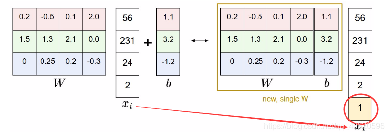
④ 简化Score求值
因为Score=W * x + b,计算则是先求出W * X再加上b,而下图左右两部分相等,只需要在x中加一个元素1,就可以将W和b组合处理。
#------------------------------svm.pyinb文件----------------------------------
# third: append the bias dimension of ones (i.e. bias trick) so that our SVM
# only has to worry about optimizing a single weight matrix W.
X_train = np.hstack([X_train, np.ones((X_train.shape[0], 1))])				# 1
X_val = np.hstack([X_val, np.ones((X_val.shape[0], 1))])
X_test = np.hstack([X_test, np.ones((X_test.shape[0], 1))])
X_dev = np.hstack([X_dev, np.ones((X_dev.shape[0], 1))])

print(X_train.shape, X_val.shape, X_test.shape, X_dev.shape)
#(49000, 3073)
#(1000, 3073)
#(1000, 3073)
#(500, 3073)
- #1:np.ones((X_val.shape[0], 1))生成一个shape=(49000,1);
- #1:将在X_train后额外添加一个全1的列,因此列数全都加1,变成3073列。
2、SVM线性分类器
对于SVM线性分类器分成以下几个步骤:
- 模型建立;
- 梯度计算和检验;
- 训练和预测;
- 权重可视化。
① 模型建立
首先最开始则是建立线性分类器,而梯度更新有两种方法
- 方法一:
#------------------------------linear_svm.py----------------------------------
def svm_loss_naive(W, X, y, reg):
  """
  Structured SVM loss function, naive implementation (with loops).

  Inputs have dimension D, there are C classes, and we operate on minibatches
  of N examples.

  Inputs:
 - W: A numpy array of shape (D, C) containing weights.
 - X: A numpy array of shape (N, D) containing a minibatch of data.
 - y: A numpy array of shape (N,) containing training labels; y[i] = c means
    that X[i] has label c, where 0 <= c < C.
 - reg: (float) regularization strength

  Returns a tuple of:
 - loss as single float
 - gradient with respect to weights W; an array of same shape as W
  """
  dW = np.zeros(W.shape) # initialize the gradient as zero

  # compute the loss and the gradient
  num_classes = W.shape[1]
  num_train = X.shape[0]
  loss = 0.0
  for i in xrange(num_train):
    scores = X[i].dot(W)     		# scores.shape -> (1,D)*(D,C)=(1,C)
    correct_class_score = scores[y[i]]
    for j in xrange(num_classes):
      if j == y[i]:
        continue					# if(1),The following statement is not executed
      margin = scores[j] - correct_class_score + 1 			# delta = 1
      if margin > 0:
        loss += margin

  # Right now the loss is a sum over all training examples, but we want it
  # to be an average instead so we divide by num_train.
  loss /= num_train
  dW /=num_train


  # Add regularization to the loss.
  loss+=0.5*reg*np.sum(W*W)
  dW+=reg*W
  #############################################################################
  # TODO:                                                                     #
  # Compute the gradient of the loss function and store it dW.                #
  # Rather that first computing the loss and then computing the derivative,   #
  # it may be simpler to compute the derivative at the same time that the     #
  # loss is being computed. As a result you may need to modify some of the    #
  # code above to compute the gradient.                                       #
  #############################################################################

  return loss, dW
- #1:表示采用数值方式计算损失函数和梯度
- reg 表示正则化系数
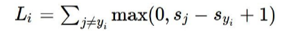
the SVM loss有如下形式:
方法二
def svm_loss_vectorized(W, X, y, reg):
  """
  Structured SVM loss function, vectorized implementation.

  Inputs and outputs are the same as svm_loss_naive.
  """
  loss = 0.0
  dW = np.zeros(W.shape) # initialize the gradient as zero

  #############################################################################
  # TODO:                                                                     #
  # Implement a vectorized version of the structured SVM loss, storing the    #
  # result in loss.                                                           #
  #############################################################################
  pass
  #############################################################################
  #                             END OF YOUR CODE                              #
  #############################################################################


  #############################################################################
  # TODO:                                                                     #
  # Implement a vectorized version of the gradient for the structured SVM     #
  # loss, storing the result in dW.                                           #
  #                                                                           #
  # Hint: Instead of computing the gradient from scratch, it may be easier    #
  # to reuse some of the intermediate values that you used to compute the     #
  # loss.                                                                     #
  #############################################################################
  pass
  #############################################################################
  #                             END OF YOUR CODE                              #
  #############################################################################
  return loss, dW
以下是KNearestNeighbor类的一部分,可以看出train方法只是将数据输入,以满足后序方法数据需要。
#------------------------k_nearest_neighbor.py文件----------------------------------
import numpy as np
from past.builtins import xrange

class KNearestNeighbor(object):
  """ a kNN classifier with L2 distance """

  def __init__(self):
    pass

  def train(self, X, y):
    """
    Train the classifier. For k-nearest neighbors this is just
    memorizing the training data.

    Inputs:
    - X: A numpy array of shape (num_train, D) containing the training data
      consisting of num_train samples each of dimension D.
    - y: A numpy array of shape (N,) containing the training labels, where
         y[i] is the label for X[i].
    """
    self.X_train = X
    self.y_train = y
3.2 计算欧式距离L2
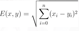
中心思想:计算第i幅测试以及第j幅训练图之间距离,将所得值保存在dists[ i ][ j ]中,结果是一个矩阵,第i行是测试图i与所有训练图之间的L2距离,所有总行数等于测试图数X_test.shape[0]=500,总列数等于训练图数X_train.shape[0]=5000。
3.2.1 用两个循环来计算欧式L2距离
At first, open cs231n/classifiers/k_nearest_neighbor.py and implement the function compute_distances_two_loops.
#------------------------k_nearest_neighbor.py文件----------------------------------
def compute_distances_two_loops(self, X):
    """
    Compute the distance between each test point in X and each training point
    in self.X_train using a nested loop over both the training data and the
    test data.

    Inputs:
    - X: A numpy array of shape (num_test, D) containing test data.

    Returns:
    - dists: A numpy array of shape (num_test, num_train) where dists[i, j]
      is the Euclidean distance between the ith test point and the jth training
      point.
    """
    num_test = X.shape[0]
    num_train = self.X_train.shape[0]
    dists = np.zeros((num_test, num_train))
    for i in xrange(num_test):              #测试样本的循环
      for j in xrange(num_train):            #训练样本的循环
        #####################################################################
        # TODO:                                                             #
        # Compute the l2 distance between the ith test point and the jth    #计算欧式距离l2
        # training point, and store the result in dists[i, j]. You should   #
        # not use a loop over dimension.                                    #
        #####################################################################

        dists[i][j] = np.sqrt(np.sum(np.square(self.X_train[j,:] - X[i,:])))

        #####################################################################
        #                       END OF YOUR CODE                            #
        #####################################################################
    return dists
3.2.2 用一个循环来计算欧式L2距离
At first, open cs231n/classifiers/k_nearest_neighbor.py and implement the function compute_distances_one_loop.
#------------------------k_nearest_neighbor.py文件----------------------------------
def compute_distances_one_loop(self, X):
    """
    Compute the distance between each test point in X and each training point
    in self.X_train using a single loop over the test data.

    Input / Output: Same as compute_distances_two_loops
    """
    num_test = X.shape[0]
    num_train = self.X_train.shape[0]
    dists = np.zeros((num_test, num_train))
    for i in xrange(num_test):
      #######################################################################
      # TODO:                                                               #
      # Compute the l2 distance between the ith test point and all training #
      # points, and store the result in dists[i, :].                        #
      #######################################################################

      dists[i,:] = np.sqrt(np.sum(np.square(self.X_train-X[i,:]),axis = 1))		# 1

      #######################################################################
      #                         END OF YOUR CODE                            #
      #######################################################################
    return dists
程序解读:
- #1:self.X_train-X[i,:]------->由于self.X_train是(5000,3072),而X[i,:]是X的第i行,即(1,3072),这个相减则是将X[i,:]延展成(5000,3072),每一行都与第一行一样,最后结果(5000,3072)就是每一幅训练图都与第i幅测试图进行相减;
- #1:np.sum(np.square(self.X_train-X[i,:]),axis = 1)--------->进行行求和,最后结果是(5000, )。
Q1: 这里我一直没想通为什么维度会改变,从原来的二维变成一维,按正常思路:将(5000,3072)进行行求和,那么结果一定是(5000,1),这个就是列向量,怎么可能赋值给行向量dists[i,:]?
Answer:后来经过尝试发现sum会自动降维,(5000,3072)进行行求和,结果是(5000, ),如果要保持维度不发生变化,则用语句np.sum(np.square(self.X_train-X[i,:]),axis = 1,keepdims=True),这时sum就不会自动降维,结果仍旧是二维,shape=(5000, 1),最后,由于结果自动降维成(5000, ),它既不是行向量也不是列向量,因此既可以赋给行向量,也可以赋给列向量。
3.2.3 不使用循环,直接计算欧式L2距离
At first, open cs231n/classifiers/k_nearest_neighbor.py and implement the function compute_distances_no_loops.
#------------------------k_nearest_neighbor.py文件----------------------------------
def compute_distances_no_loops(self, X):
    """
    Compute the distance between each test point in X and each training point
    in self.X_train using no explicit loops.

    Input / Output: Same as compute_distances_two_loops
    """
    num_test = X.shape[0]
    num_train = self.X_train.shape[0]
    dists = np.zeros((num_test, num_train))
    #########################################################################
    # TODO:                                                                 #
    # Compute the l2 distance between all test points and all training      #
    # points without using any explicit loops, and store the result in      #
    # dists.                                                                #
    #                                                                       #
    # You should implement this function using only basic array operations; #
    # in particular you should not use functions from scipy.                #
    #                                                                       #
    # HINT: Try to formulate the l2 distance using matrix multiplication    #
    #       and two broadcast sums.                                         #
    #########################################################################

    mul1 = np.multiply(np.dot(X,self.X_train.T),-2)   							# 1
    sq1 = np.sum(np.square(X),axis=1,keepdims = True)   						# 2
    sq2 = np.sum(np.square(self.X_train),axis=1)   								# 3
    dists = mul1+sq1+sq2
    dists = np.sqrt(dists)                  #通过 x^2 - 2xy + y^2 = (x-y)^2 来实现

    #########################################################################
    #                         END OF YOUR CODE                              #
    #########################################################################
    return dists
程序解读:
- #1:相当于求 " -2xy ";
- #2:相当于求" x^2 ";
- #3:相当于求" y^2 "。
最后结果可以知道mul1.shape=(500,5000),sq1.shape=(500,1),sq2.shape=(5000, )
Q2: 三个规格不相同的向量进行相加,怎么进行?
Answer:还是通过尝试发现(sq1+sq2).shape=(500,5000)
Eg:一维向量和列向量相加的运算!!!
In :       	c = np.array([1,2,3,4])          		#c.shape = (4, )
Out: 		[1 2 3 4]

In :       	a = c.reshape((4,1))          			#a.shape = (4,1)
Out: 		[[1]
 			 [2]
			 [3]
			 [4]]

In :       	print(c+a)          					#(c+a).shape = (4,4)
Out:		[[2 3 4 5]
 			 [3 4 5 6]
			 [4 5 6 7]
			 [5 6 7 8]]
3.3 分类器预测
#------------------------k_nearest_neighbor.py文件----------------------------------
def predict_labels(self, dists, k=1):
    """
    Given a matrix of distances between test points and training points,
    predict a label for each test point.

    Inputs:
    - dists: A numpy array of shape (num_test, num_train) where dists[i, j]
      gives the distance betwen the ith test point and the jth training point.

    Returns:
    - y: A numpy array of shape (num_test,) containing predicted labels for the
      test data, where y[i] is the predicted label for the test point X[i].
    """
    num_test = dists.shape[0]
    y_pred = np.zeros(num_test)
    for i in xrange(num_test):
      # A list of length k storing the labels of the k nearest neighbors to
      # the ith test point.
      closest_y = []
      #########################################################################
      # TODO:                                                                 #
      # Use the distance matrix to find the k nearest neighbors of the ith    #
      # testing point, and use self.y_train to find the labels of these       #
      # neighbors. Store these labels in closest_y.                           #
      # Hint: Look up the function numpy.argsort.                             #
      #########################################################################
      closest_y = self.y_train[np.argsort(dists[i,:])[:k]]  							# 1
      #########################################################################
      # TODO:                                                                 #
      # Now that you have found the labels of the k nearest neighbors, you    #
      # need to find the most common label in the list closest_y of labels.   #
      # Store this label in y_pred[i]. Break ties by choosing the smaller     #
      # label.                                                                #
      #########################################################################
      y_pred[i] = np.argmax(np.bincount(closest_y))										# 2
      #########################################################################
      #                           END OF YOUR CODE                            #
      #########################################################################

    return y_pred
程序解读:
- #1:np.argsort(dists[i,:])[:k] :将dists第i行的数值进行处理,将该行元素值从小到大排序(为什么从小到大?因为越小说明越相近),然后返回它们索引值来组成一个数组(1,5000),最后取前k列;目的在于选k张与测试图片最相近的训练图片出来。其中closest_y (1, k);
- #1:self.y_train[np.argsort(dists[i,:])[:k]]:这个将得到这k张训练图片的label值;
- #2:np.bincount(closest_y):得到所有索引值(种类如果是k+1种,则索引值0~k)在closest_y中出现的次数,将次数组成一个数组,故大小则是(1,k+1);
- #2:np.argmax(np.bincount(closest_y)):argmax用来求出数组中元素最大值所对应的索引,因此返回一个值,该值则是最终预测的label的索引值,其实索引值就是label值,返回索引就够了,没必要转成label名称,最后存到y_pred[i]中。
4、KNN结果展示
4.1 用颜色深浅形式查看dists元素值
#------------------------------knn文件----------------------------------
# We can visualize the distance matrix: each row is a single test example and
# its distances to training examples
plt.imshow(dists, interpolation='none')
plt.show()
上述代码中interpolation代表的是插值运算,'none’是选取的是不插值方式,将dists的每个元素展示出来,结果如下:
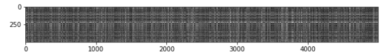
从上面图片看,如果第i行越黑,则说明第i张测试图和所有训练图相似,越亮则越不相似;若第j列越黑则说明第j张训练图和所有测试图越相似
4.2 计算准确度(k=1)
#------------------------------knn文件----------------------------------
# Now implement the function predict_labels and run the code below:
# We use k = 1 (which is Nearest Neighbor).
y_test_pred = classifier.predict_labels(dists, k=1)

# Compute and print the fraction of correctly predicted examples
num_correct = np.sum(y_test_pred == y_test)
accuracy = float(num_correct) / num_test
print('Got %d / %d correct => accuracy: %f' % (num_correct, num_test, accuracy))
程序解读:
- 先令k=1,即最近邻为1;
- 将这500张测试图片预测完label后,与准确的label值进行比较,若一样则得分为1,不一样则得分为0,最后除以500,得到的就是准确度。
4.3 计算准确度(k=5)
#------------------------------knn文件----------------------------------
y_test_pred = classifier.predict_labels(dists, k=5)
num_correct = np.sum(y_test_pred == y_test)
accuracy = float(num_correct) / num_test
print('Got %d / %d correct => accuracy: %f' % (num_correct, num_test, accuracy))
程序解读:
- 再令k=5,最近邻改为5,重复之前k=1的工作;
- 将这500张测试图片预测完label后,与准确的label值进行比较,若一样则得分为1,不一样则得分为0,最后除以500,得到的就是准确度。
5、交叉验证确定k值
之前我们已经实现了k近邻分类器,但是我们是随意设置 k 的值。接下来我们将通过交叉验证来确定这个超参数的最佳值。我们采用S折交叉验证的方法,即将数据平均分成S份,一份作为测试集,其余作为训练集,一般S=10,本文将S设为5,即代码中num_folds = 5。
5.1 交叉验证
#------------------------------knn文件----------------------------------
num_folds = 5
k_choices = [1, 3, 5, 8, 10, 12, 15, 20, 50, 100]

X_train_folds = []
y_train_folds = []
################################################################################
# TODO:                                                                        #
# Split up the training data into folds. After splitting, X_train_folds and    #
# y_train_folds should each be lists of length num_folds, where                #
# y_train_folds[i] is the label vector for the points in X_train_folds[i].     #
# Hint: Look up the numpy array_split function.                                #
################################################################################
y_train_ = y_train.reshape(-1, 1)
X_train_folds = np.array_split(X_train, 5)                                  # 1
y_train_folds = np.array_split(y_train_, 5)
################################################################################
#                                 END OF YOUR CODE                             #
################################################################################

# A dictionary holding the accuracies for different values of k that we find
# when running cross-validation. After running cross-validation,
# k_to_accuracies[k] should be a list of length num_folds giving the different
# accuracy values that we found when using that value of k.
k_to_accuracies = {}                                                        # 2


################################################################################
# TODO:                                                                        #
# Perform k-fold cross validation to find the best value of k. For each        #
# possible value of k, run the k-nearest-neighbor algorithm num_folds times,   #
# where in each case you use all but one of the folds as training data and the #
# last fold as a validation set. Store the accuracies for all fold and all     #
# values of k in the k_to_accuracies dictionary.                               #
################################################################################
for k_ in k_choices:
    k_to_accuracies.setdefault(k_, [])
for i in range(num_folds):												    # 3
    classifier = KNearestNeighbor()
    X_val_train = np.vstack(X_train_folds[0:i] + X_train_folds[i+1:])       # 4
    y_val_train = np.vstack(y_train_folds[0:i] + y_train_folds[i+1:])
    y_val_train = y_val_train[:,0]
    classifier.train(X_val_train, y_val_train)
    for k_ in k_choices:
        y_val_pred = classifier.predict(X_train_folds[i], k=k_)			    # 5
        num_correct = np.sum(y_val_pred == y_train_folds[i][:,0])
        accuracy = float(num_correct) / len(y_val_pred)
        k_to_accuracies[k_] = k_to_accuracies[k_] + [accuracy]
################################################################################
#                                 END OF YOUR CODE                             #
################################################################################

# Print out the computed accuracies
for k in sorted(k_to_accuracies):										    # 6
    for accuracy in k_to_accuracies[k]:
        print('k = %d, accuracy = %f' % (k, accuracy))
程序解读:
- #1:表示将数据训练集平均分成5份,对应的标签也分为5份;
- #2:以字典形式存储k 和accuracy;
- #3:依次对每个k (1,3,5,8,10,12,15,20,50,100)值,选取一份测试,其余训练,计算准确率,由于之前平均分为5份,故对每个k都有五个结果;
- #4:表示除 i 之外的作为训练集;
- #5:将第 i 份作为测试集并预测;
- #6:输出每个k值五次得到的准确率。
结果:
k = 1, accuracy = 0.263000
k = 1, accuracy = 0.257000
k = 1, accuracy = 0.264000
k = 1, accuracy = 0.278000
k = 1, accuracy = 0.266000
k = 3, accuracy = 0.239000
k = 3, accuracy = 0.249000
k = 3, accuracy = 0.240000
k = 3, accuracy = 0.266000
k = 3, accuracy = 0.254000
k = 5, accuracy = 0.248000
k = 5, accuracy = 0.266000
k = 5, accuracy = 0.280000
k = 5, accuracy = 0.292000
k = 5, accuracy = 0.280000
k = 8, accuracy = 0.262000
k = 8, accuracy = 0.282000
k = 8, accuracy = 0.273000
k = 8, accuracy = 0.290000
k = 8, accuracy = 0.273000
k = 10, accuracy = 0.265000
k = 10, accuracy = 0.296000
k = 10, accuracy = 0.276000
k = 10, accuracy = 0.284000
k = 10, accuracy = 0.280000
k = 12, accuracy = 0.260000
k = 12, accuracy = 0.295000
k = 12, accuracy = 0.279000
k = 12, accuracy = 0.283000
k = 12, accuracy = 0.280000
k = 15, accuracy = 0.252000
k = 15, accuracy = 0.289000
k = 15, accuracy = 0.278000
k = 15, accuracy = 0.282000
k = 15, accuracy = 0.274000
k = 20, accuracy = 0.270000
k = 20, accuracy = 0.279000
k = 20, accuracy = 0.279000
k = 20, accuracy = 0.282000
k = 20, accuracy = 0.285000
k = 50, accuracy = 0.271000
k = 50, accuracy = 0.288000
k = 50, accuracy = 0.278000
k = 50, accuracy = 0.269000
k = 50, accuracy = 0.266000
k = 100, accuracy = 0.256000
k = 100, accuracy = 0.270000
k = 100, accuracy = 0.263000
k = 100, accuracy = 0.256000
k = 100, accuracy = 0.263000
5.2 结果展示
将每个k下的五个准确率求平均后,用图片展示,从图中就可以直观看出k的最佳值,如图,当k=10 时,准确率最高。
#------------------------------knn文件----------------------------------
# plot the raw observations
for k in k_choices:
    accuracies = k_to_accuracies[k]
    plt.scatter([k] * len(accuracies), accuracies)

# plot the trend line with error bars that correspond to standard deviation
accuracies_mean = np.array([np.mean(v) for k,v in sorted(k_to_accuracies.items())])
accuracies_std = np.array([np.std(v) for k,v in sorted(k_to_accuracies.items())])
plt.errorbar(k_choices, accuracies_mean, yerr=accuracies_std)
plt.title('Cross-validation on k')
plt.xlabel('k')
plt.ylabel('Cross-validation accuracy')
plt.show()

