cs231n assignment1：KNN/SVM/Softmax/Two_layer_net

一、knn:

1.knn.py中实现

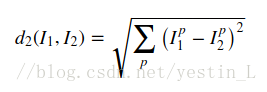
a.分别用双重循环、单重循环和不使用循环实现欧式距离公式

 公式：

双重循环：

  def compute_distances_two_loops(self, X):
    """
    Compute the distance between each test point in X and each training point
    in self.X_train using a nested loop over both the training data and the 
    test data.

    Inputs:
    - X: A numpy array of shape (num_test, D) containing test data.

    Returns:
    - dists: A numpy array of shape (num_test, num_train) where dists[i, j]
      is the Euclidean distance between the ith test point and the jth training
      point.
    """
    num_test = X.shape[0]
    num_train = self.X_train.shape[0]
    dists = np.zeros((num_test, num_train))
    for i in xrange(num_test):
      for j in xrange(num_train):
        #####################################################################
        # TODO:                                                             #
        # Compute the l2 distance between the ith test point and the jth    #
        # training point, and store the result in dists[i, j]. You should   #
        # not use a loop over dimension.                                    #
        #####################################################################
        dists[i,j] = np.sqrt(np.sum(np.square(self.X_train[j,:] - X[i,:])))
        #####################################################################
        #                       END OF YOUR CODE                            #
        #####################################################################
    return dists

单重循环：

  def compute_distances_one_loop(self, X):
    """
    Compute the distance between each test point in X and each training point
    in self.X_train using a single loop over the test data.

    Input / Output: Same as compute_distances_two_loops
    """
    num_test = X.shape[0]
    num_train = self.X_train.shape[0]
    dists = np.zeros((num_test, num_train))
    for i in xrange(num_test):
      #######################################################################
      # TODO:                                                               #
      # Compute the l2 distance between the ith test point and all training #
      # points, and store the result in dists[i, :].                        #
      #######################################################################
      dists[i,:] = np.sqrt(np.sum(np.square(self.X_train - X[i,:]),axis = 1))
      #######################################################################
      #                         END OF YOUR CODE                            #
      #######################################################################
    return dists

代码部分

  def compute_distances_no_loops(self, X):
    """
    Compute the distance between each test point in X and each training point
    in self.X_train using no explicit loops.

    Input / Output: Same as compute_distances_two_loops
    """
    num_test = X.shape[0]
    num_train = self.X_train.shape[0]
    dists = np.zeros((num_test, num_train)) 
    #########################################################################
    # TODO:                                                                 #
    # Compute the l2 distance between all test points and all training      #
    # points without using any explicit loops, and store the result in      #
    # dists.                                                                #
    #                                                                       #
    # You should implement this function using only basic array operations; #
    # in particular you should not use functions from scipy.                #
    #                                                                       #
    # HINT: Try to formulate the l2 distance using matrix multiplication    #
    #       and two broadcast sums.                                         #
    #########################################################################
    dist1 = np.sum(np.square(self.X_train),axis=1)
    dist2 = np.sum(np.square(X),axis=1)
    dist3 = np.dot(X,self.X_train.T)
    dists = np.sqrt(-2*dist3+dist1+dist2.reshape(dist2.shape[0],1))
    #########################################################################
    #                         END OF YOUR CODE                              #
    #########################################################################
    return dists

公式推导：

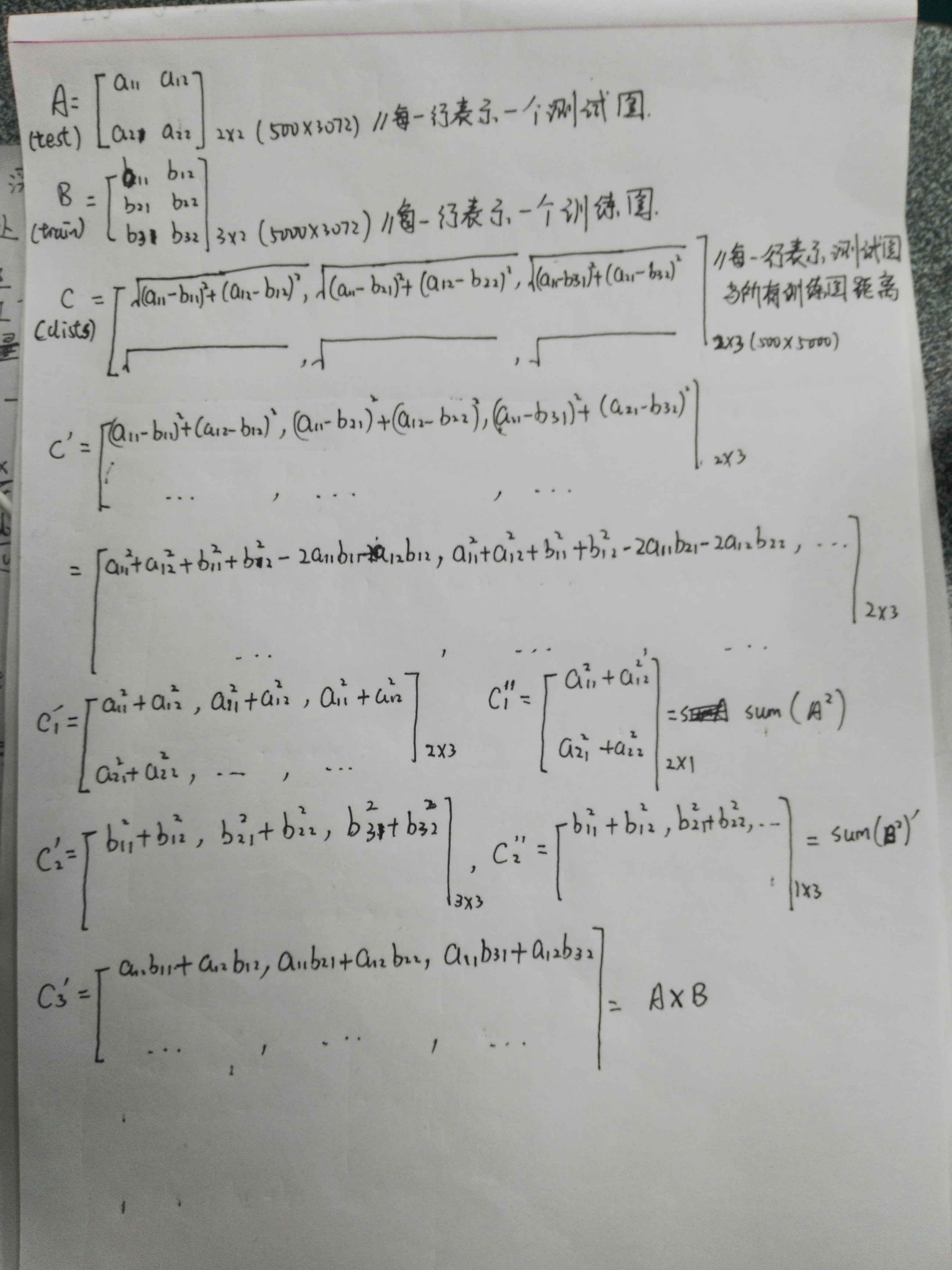
此处参考了https://www.2cto.com/kf/201710/693091.html

b.使用knn方法实现类别预测

完整代码：

  def predict_labels(self, dists, k=1):
    """
    Given a matrix of distances between test points and training points,
    predict a label for each test point.

    Inputs:
    - dists: A numpy array of shape (num_test, num_train) where dists[i, j]
      gives the distance betwen the ith test point and the jth training point.

    Returns:
    - y: A numpy array of shape (num_test,) containing predicted labels for the
      test data, where y[i] is the predicted label for the test point X[i].  
    """
    num_test = dists.shape[0]
    y_pred = np.zeros(num_test)
    for i in xrange(num_test):

      # A list of length k storing the labels of the k nearest neighbors to
      # the ith test point.
      closest_y = []
      #########################################################################
      # TODO:                                                                 #
      # Use the distance matrix to find the k nearest neighbors of the ith    #
      # testing point, and use self.y_train to find the labels of these       #
      # neighbors. Store these labels in closest_y.                           #
      # Hint: Look up the function numpy.argsort.                             #
      #########################################################################
      closest_y = self.y_train[np.argsort(dists[i,:])[:k]]
      #########################################################################
      # TODO:                                                                 #
      # Now that you have found the labels of the k nearest neighbors, you    #
      # need to find the most common label in the list closest_y of labels.   #
      # Store this label in y_pred[i]. Break ties by choosing the smaller     #
      # label.                                                                #
      #########################################################################
      y_pred[i] = np.argmax(np.bincount(closest_y))
      #########################################################################
      #                           END OF YOUR CODE                            # 
      #########################################################################

    return y_pred    

代码解析：

 closest_y = self.y_train[np.argsort(dists[i,:])[:k]]

用np.argsort函数实现对现在的dists每一行从小到大排序,返回相应的所在切片的值。同时获取训练值中y标签前k个对应切片位置的类别值，并存入用y_pred的相应行中。

 y_pred[i] = np.argmax(np.bincount(closest_y))

用np.bincount函数统计closest_y相同值的数量，并填入相应的切片位。然后用argmax提取出切片位，该值为统计量最高的类别值。

2.knn.ipynb代码实现

Cross Validation

num_folds = 5
k_choices = [1, 3, 5, 8, 10, 12, 15, 20, 50, 100]

X_train_folds = []
y_train_folds = []
################################################################################
# TODO:                                                                        #
# Split up the training data into folds. After splitting, X_train_folds and    #
# y_train_folds should each be lists of length num_folds, where                #
# y_train_folds[i] is the label vector for the points in X_train_folds[i].     #
# Hint: Look up the numpy array_split function.                                #
################################################################################
X_train_folds = np.array_split(X_train,num_folds)
y_train_folds = np.array_split(y_train,num_folds)
################################################################################
#                                 END OF YOUR CODE                             #
################################################################################

# A dictionary holding the accuracies for different values of k that we find
# when running cross-validation. After running cross-validation,
# k_to_accuracies[k] should be a list of length num_folds giving the different
# accuracy values that we found when using that value of k.
k_to_accuracies = {}



################################################################################
# TODO:                                                                        #
# Perform k-fold cross validation to find the best value of k. For each        #
# possible value of k, run the k-nearest-neighbor algorithm num_folds times,   #
# where in each case you use all but one of the folds as training data and the #
# last fold as a validation set. Store the accuracies for all fold and all     #
# values of k in the k_to_accuracies dictionary.                               #
################################################################################

for k in k_choices:
    k_to_accuracies[k] = np.zeros(num_folds)
    for i in range(num_folds):
        Xtr = np.array(X_train_folds[:i]+X_train_folds[i+1:])
        Xte = np.array(X_train_folds[i])
        ytr = np.array(y_train_folds[:i]+y_train_folds[i+1:])
        yte = np.array(y_train_folds[i]) 
        
        #reshape the training and test array
        Xtr = np.reshape(Xtr,(Xtr.shape[0]*Xtr.shape[1],-1))
        ytr = np.reshape(ytr,(ytr.shape[0]*ytr.shape[1],-1))
        ytr = np.reshape(ytr,len(ytr)) #flatten the shape of ytr into  1*4000
        
        classifier.train(Xtr,ytr)
        yte_pred = classifier.predict(Xte,k)
        num_correct = np.sum(yte_pred == yte)
        accuracy = float(num_correct) / len(yte)
        k_to_accuracies[k][i] = accuracy
        
################################################################################
#                                 END OF YOUR CODE                             #
################################################################################

# Print out the computed accuracies
for k in sorted(k_to_accuracies):
    for accuracy in k_to_accuracies[k]:
        print('k = %d, accuracy = %f' % (k, accuracy))

参考链接：https://blog.csdn.net/MargretWG/article/details/69056256

代码详解：

X_train_folds = np.array_split(X_train,num_folds)
y_train_folds = np.array_split(y_train,num_folds)

用np.array_split函数将训练集和标签均分成5份，用于交叉验证

for k in k_choices:                                            #试k的值，寻找最优k值
    k_to_accuracies[k] = np.zeros(num_folds)                   #让字典中的key值为不同k值，且一个key对应5个值
    for i in range(num_folds):                                 #让分类的训练集循环做测试集
        Xtr = np.array(X_train_folds[:i]+X_train_folds[i+1:])  #将第i个训练集做测试集，其余做训练集
        Xte = np.array(X_train_folds[i])                       #Xtr.shape=(4,1000,3072) Xte.shape=(1000,3072)
        ytr = np.array(y_train_folds[:i]+y_train_folds[i+1:])  #ytr.shape=(1000,) yte.shape=(4,1000,1)               
        yte = np.array(y_train_folds[i])                                             
        
        #reshape the training and test array
        Xtr = np.reshape(Xtr,(Xtr.shape[0]*Xtr.shape[1],-1))   #Xtr.shape=(4000,3072)
        ytr = np.reshape(ytr,(ytr.shape[0]*ytr.shape[1],-1))   #ytr.shape=(4000,1)
        ytr = np.reshape(ytr,len(ytr)) #flatten the shape of ytr into  1*4000
                                                               #ytr.shape=(4000,)
        classifier.train(Xtr,ytr)                              #输入训练集
        yte_pred = classifier.predict(Xte,k)                   #预测标签并返回，使用无循环
        num_correct = np.sum(yte_pred == yte)                
        accuracy = float(num_correct) / len(yte)                    
        k_to_accuracies[k][i] = accuracy                       #将准确值存入

参考链接中缺了红色字体的部分代码，输出会报错

#ValueError: object too deep for desired array

加上红色部分代码就可以。这是因为如果不加上的话，ytr.shape是一个4000*1的二维矩阵，我试过输入代码

ytr = np.reshape(ytr,(-1,ytr.shape[0]*ytr.shape[1]))

    这样也不行，虽然这样返回的是一个1*4000的矩阵，但这个在numpy里会被认为是二维的矩阵，而不是我们直观上的一维行向量。如果用print(ytr) ，会等于[ [ ....] ] 的一个二维矩阵。只有再reshape(ytr,len(ytr))时才能将二维矩阵化为一个一维的，这时再print(ytr),就会输出[...]的一个一维行向量。

    而且还要注意的一点是，len（）返回的是矩阵的行数量，所以这里要先把ytr变成4000*1的二维矩阵，而非1*4000的。

    总之一定要注意输入参数的维度。

二、SVM

1.linear_svm.py代码实现及推导

a.svm_loss_naive

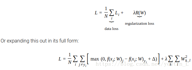
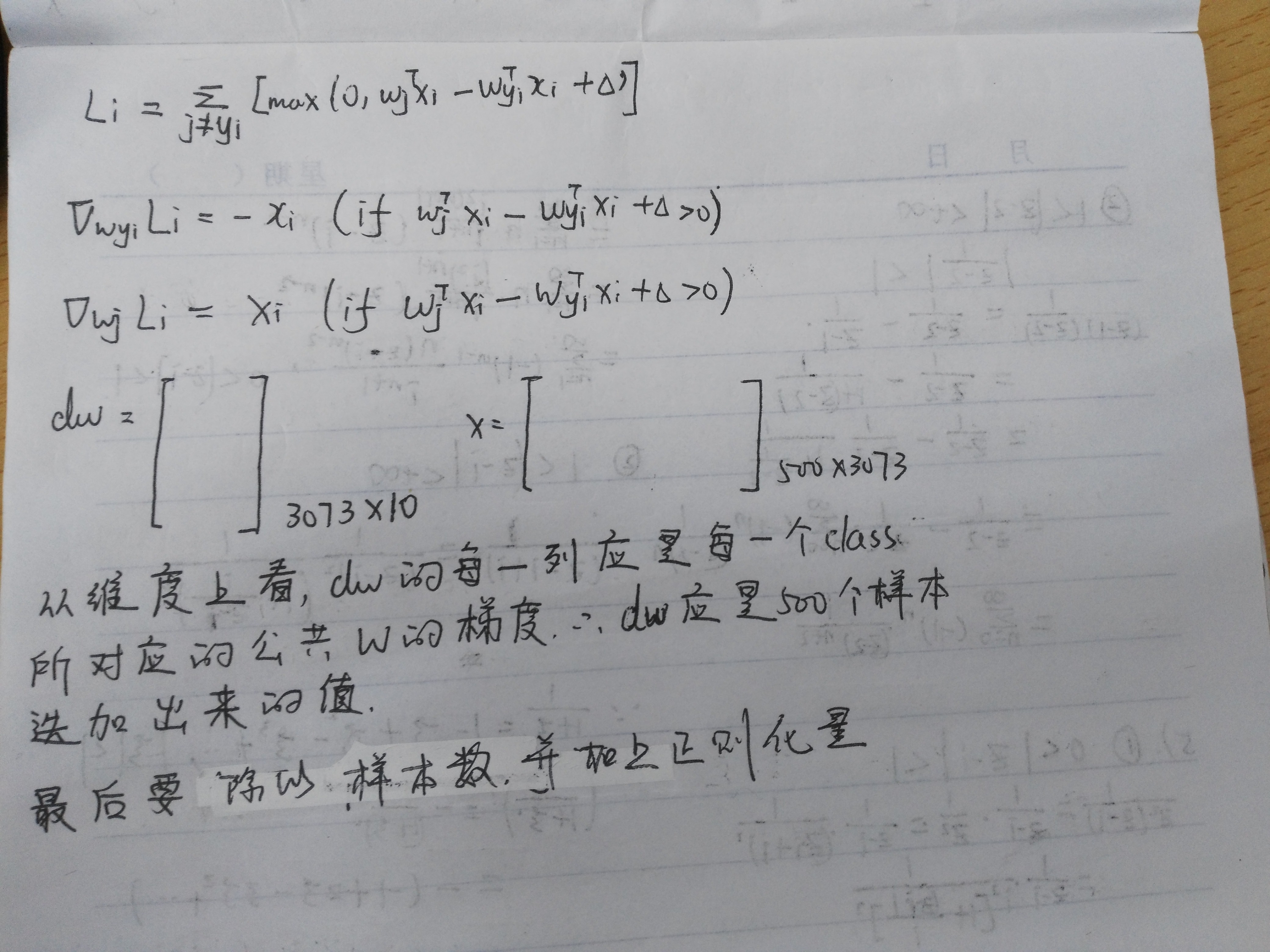
loss部分比较简单，代码已经给出，就是完成公式

 即可

                                                                        (使用L2正则化损失项）

计算gradient并存入dW中

代码：

def svm_loss_naive(W, X, y, reg):
  """
  Structured SVM loss function, naive implementation (with loops).

  Inputs have dimension D, there are C classes, and we operate on minibatches
  of N examples.

  Inputs:
  - W: A numpy array of shape (D, C) containing weights.
  - X: A numpy array of shape (N, D) containing a minibatch of data.
  - y: A numpy array of shape (N,) containing training labels; y[i] = c means
    that X[i] has label c, where 0 <= c < C.
  - reg: (float) regularization strength

  Returns a tuple of:
  - loss as single float
  - gradient with respect to weights W; an array of same shape as W
  """
  dW = np.zeros(W.shape) # initialize the gradient as zero

  # compute the loss and the gradient
  num_classes = W.shape[1]
  num_train = X.shape[0]
  loss = 0.0
  for i in xrange(num_train):
    scores = X[i].dot(W)
    correct_class_score = scores[y[i]]
    for j in xrange(num_classes):
      if j == y[i]:
        continue
      margin = scores[j] - correct_class_score + 1 # note delta = 1
      if margin > 0:
        loss += margin
        dW[:,y[i]] += -X[i,:].T
        dW[:,j] += X[i,].T

  # Right now the loss is a sum over all training examples, but we want it
  # to be an average instead so we divide by num_train.
  loss /= num_train
  dW /= num_train
  # Add regularization to the loss.
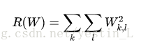
  loss += reg * np.sum(W * W)
  dW += reg*W

推导

b.svm_loss_vectorized

def svm_loss_vectorized(W, X, y, reg):
  """
  Structured SVM loss function, vectorized implementation.

  Inputs and outputs are the same as svm_loss_naive.
  """
  loss = 0.0
  dW = np.zeros(W.shape) # initialize the gradient as zero
  num_train = X.shape[0]
  #############################################################################
  # TODO:                                                                     #
  # Implement a vectorized version of the structured SVM loss, storing the    #
  # result in loss.                                                           #
  #############################################################################
  scores = X.dot(W)
  correct_class_score = scores[np.arange(num_train), y]
  correct_class_score = np.reshape(correct_class_score,(num_train,-1))
  margins = scores - correct_class_score + 1.0
  margins[np.arange(num_train),y] = 0.0
  margins[margins <= 0] = 0.0
  loss += np.sum(margins) / num_train
  loss += reg*np.sum(W*W)
  #############################################################################
  #                             END OF YOUR CODE                              #
  #############################################################################


  #############################################################################
  # TODO:                                                                     #
  # Implement a vectorized version of the gradient for the structured SVM     #
  # loss, storing the result in dW.                                           #
  #                                                                           #
  # Hint: Instead of computing the gradient from scratch, it may be easier    #
  # to reuse some of the intermediate values that you used to compute the     #
  # loss.                                                                     #
  #############################################################################
  margins[margins > 0] = 1.0
  row_sum = np.sum(margins,axis=1)
  margins[np.arange(num_train), y] = -row_sum
  dW += np.dot(X.T, margins) / num_train + reg*W
  #############################################################################
  #                             END OF YOUR CODE                              #
  #############################################################################

  return loss, dW

原理同上，这里只是去掉了循环，将操作矩阵化了，使代码运行效率更高

2.linear_classifier.py代码实现及推导

a.train函数

训练后得到权重矩阵存入self.W中

代码

  def train(self, X, y, learning_rate=1e-3, reg=1e-5, num_iters=100,
            batch_size=200, verbose=False):
    """
    Train this linear classifier using stochastic gradient descent.

    Inputs:
    - X: A numpy array of shape (N, D) containing training data; there are N
      training samples each of dimension D.
    - y: A numpy array of shape (N,) containing training labels; y[i] = c
      means that X[i] has label 0 <= c < C for C classes.
    - learning_rate: (float) learning rate for optimization.
    - reg: (float) regularization strength.
    - num_iters: (integer) number of steps to take when optimizing
    - batch_size: (integer) number of training examples to use at each step.
    - verbose: (boolean) If true, print progress during optimization.

    Outputs:
    A list containing the value of the loss function at each training iteration.
    """
    num_train, dim = X.shape
    num_classes = np.max(y) + 1 # assume y takes values 0...K-1 where K is number of classes
    if self.W is None:
      # lazily initialize W
      self.W = 0.001 * np.random.randn(dim, num_classes)

    # Run stochastic gradient descent to optimize W
    loss_history = []
    for it in xrange(num_iters):
      X_batch = None
      y_batch = None

      #########################################################################
      # TODO:                                                                 #
      # Sample batch_size elements from the training data and their           #
      # corresponding labels to use in this round of gradient descent.        #
      # Store the data in X_batch and their corresponding labels in           #
      # y_batch; after sampling X_batch should have shape (dim, batch_size)   #
      # and y_batch should have shape (batch_size,)                           #
      #                                                                       #
      # Hint: Use np.random.choice to generate indices. Sampling with         #
      # replacement is faster than sampling without replacement.              #
      #########################################################################
      sample_index = np.random.choice(num_train,batch_size,replace = False)
      X_batch = X[sample_index,:]
      y_batch = y[sample_index]
      #########################################################################
      #                       END OF YOUR CODE                                #
      #########################################################################

      # evaluate loss and gradient
      loss, grad = self.loss(X_batch, y_batch, reg)
      loss_history.append(loss)

      # perform parameter update
      #########################################################################
      # TODO:                                                                 #
      # Update the weights using the gradient and the learning rate.          #
      #########################################################################
      self.W -= learning_rate*grad
      #########################################################################
      #                       END OF YOUR CODE                                #
      #########################################################################

      if verbose and it % 100 == 0:
        print('iteration %d / %d: loss %f' % (it, num_iters, loss))

    return loss_history

代码解析：

      sample_index = np.random.choice(num_train,batch_size,replace = False)
      X_batch = X[sample_index,:]
      y_batch = y[sample_index]

用np.random.choice函数从500个训练集中随机挑选batch_size个样本及其标签

self.W -= learning_rate*grad

更新权重值

b.predict

代码：

  def predict(self, X):
    """
    Use the trained weights of this linear classifier to predict labels for
    data points.

    Inputs:
    - X: A numpy array of shape (N, D) containing training data; there are N
      training samples each of dimension D.

    Returns:
    - y_pred: Predicted labels for the data in X. y_pred is a 1-dimensional
      array of length N, and each element is an integer giving the predicted
      class.
    """
    y_pred = np.zeros(X.shape[0])
    ###########################################################################
    # TODO:                                                                   #
    # Implement this method. Store the predicted labels in y_pred.            #
    ###########################################################################
    score = X.dot(self.W)
    y_pred = np.argmax(score,axis=1)
    ###########################################################################
    #                           END OF YOUR CODE                              #
    ###########################################################################
    return y_pred

将X与W相乘获得相应的score，然后获取最大分数所对应的类别

3.svm.ipynb

用validation集去测试训练集所获得的hyperparameters，并记录相应得分，取最高得分的hypermeters作为最终的参数

# Use the validation set to tune hyperparameters (regularization strength and
# learning rate). You should experiment with different ranges for the learning
# rates and regularization strengths; if you are careful you should be able to
# get a classification accuracy of about 0.4 on the validation set.
learning_rates = [1.8e-7, 1.9e-7, 2e-7, 2.1e-7, 2.2e-7]
regularization_strengths = [2.3e4,2.4e4,2.5e4, 2.6e4, 2.7e4]

# results is dictionary mapping tuples of the form
# (learning_rate, regularization_strength) to tuples of the form
# (training_accuracy, validation_accuracy). The accuracy is simply the fraction
# of data points that are correctly classified.
results = {}
best_val = -1   # The highest validation accuracy that we have seen so far.
best_svm = None # The LinearSVM object that achieved the highest validation rate.

################################################################################
# TODO:                                                                        #
# Write code that chooses the best hyperparameters by tuning on the validation #
# set. For each combination of hyperparameters, train a linear SVM on the      #
# training set, compute its accuracy on the training and validation sets, and  #
# store these numbers in the results dictionary. In addition, store the best   #
# validation accuracy in best_val and the LinearSVM object that achieves this  #
# accuracy in best_svm.                                                        #
#                                                                              #
# Hint: You should use a small value for num_iters as you develop your         #
# validation code so that the SVMs don't take much time to train; once you are #
# confident that your validation code works, you should rerun the validation   #
# code with a larger value for num_iters.                                      #
################################################################################
iters = 3000
for lr in learning_rates:
    for rs in regularization_strengths:
        svm.train(X_train, y_train, learning_rate=lr, reg=rs, num_iters=iters)
        y_train_pred = svm.predict(X_train)
        accu_train = np.mean(y_train==y_train_pred)
        y_val_pred = svm.predict(X_val)
        accu_val = np.mean(y_val==y_val_pred)
        results[(lr,rs)] = (accu_train, accu_val)
        if best_val < accu_val:
            best_val = accu_val
            best_svm = svm
################################################################################
#                              END OF YOUR CODE                                #
################################################################################
    
# Print out results.
for lr, reg in sorted(results):
    train_accuracy, val_accuracy = results[(lr, reg)]
    print('lr %e reg %e train accuracy: %f val accuracy: %f' % (
                lr, reg, train_accuracy, val_accuracy))
    
print('best validation accuracy achieved during cross-validation: %f' % best_val)

两重循环，用不同的learning_rate和regularization_strength去训练，并将训练后获得的最优准确值更新，代码相对好理解。这里需要注意的地方就是如果直接用以上代码花费的时间会较长，最好先用题目给的两个learning_rate和regularization_strength，且将iters调小，得到相对优的解后，再不断将优解附近的learning_rate和regularization_strength细化，同时将迭代次数iters增加。

最后得到的最优准确度在3.9~4.0左右。

三、softmax

1.softmax.py

a.softmax_loss_naive函数代码实现及推导

代码：

def softmax_loss_naive(W, X, y, reg):
  """
  Softmax loss function, naive implementation (with loops)

  Inputs have dimension D, there are C classes, and we operate on minibatches
  of N examples.

  Inputs:
  - W: A numpy array of shape (D, C) containing weights.
  - X: A numpy array of shape (N, D) containing a minibatch of data.
  - y: A numpy array of shape (N,) containing training labels; y[i] = c means
    that X[i] has label c, where 0 <= c < C.
  - reg: (float) regularization strength

  Returns a tuple of:
  - loss as single float
  - gradient with respect to weights W; an array of same shape as W
  """
  # Initialize the loss and gradient to zero.
  loss = 0.0
  dW = np.zeros_like(W)

  #############################################################################
  # TODO: Compute the softmax loss and its gradient using explicit loops.     #
  # Store the loss in loss and the gradient in dW. If you are not careful     #
  # here, it is easy to run into numeric instability. Don't forget the        #
  # regularization!                                                           #
  #############################################################################
  num_train = X.shape[0]
  num_classes = W.shape[1]
  for i in xrange(num_train):
    scores = X[i].dot(W)
    scores -= np.max(scores)
    correct_class_score = scores[y[i]]
    loss += -correct_class_score + np.log(np.sum(np.exp(scores)))
    dW[:,y[i]] -= X[i].T
    for j in xrange(num_classes):
      dW[:,j] += X[i].T.dot(np.exp(scores[j])/(np.sum(np.exp(scores))))
  loss /= num_train
  loss += reg*np.sum(W*W)
  dW /= num_train
  dW += reg*W
  #############################################################################
  #                          END OF YOUR CODE                                 #
  #############################################################################

  return loss, dW

代码解析：

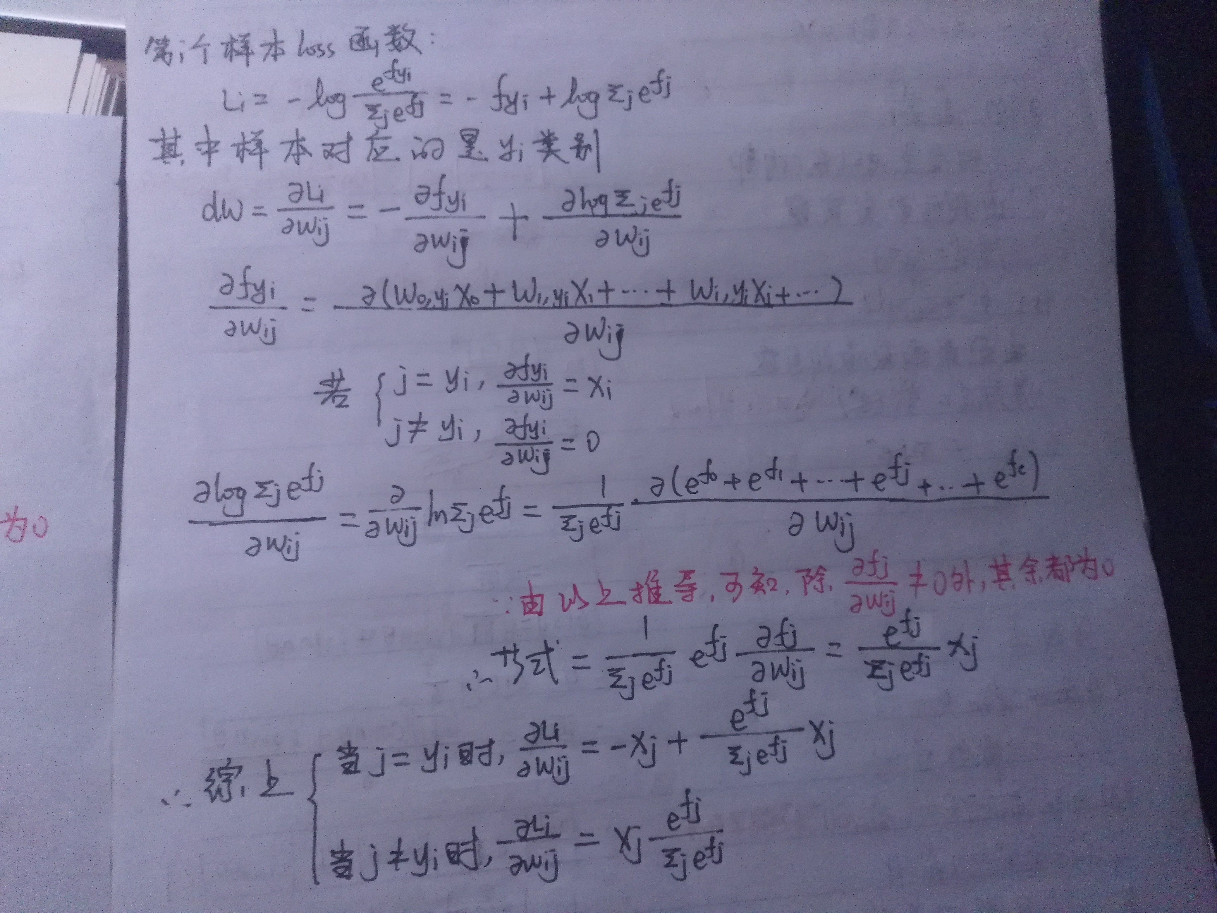
loss函数实现公式

                                                                    

                                                                    (使用L2正则化损失项）

                                

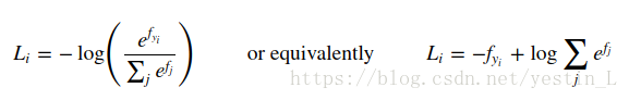
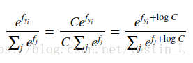
loss函数的代码比较好理解，只是要注意归一化，这里用了所有值减去最大值的办法

                                                          

                                                令                      

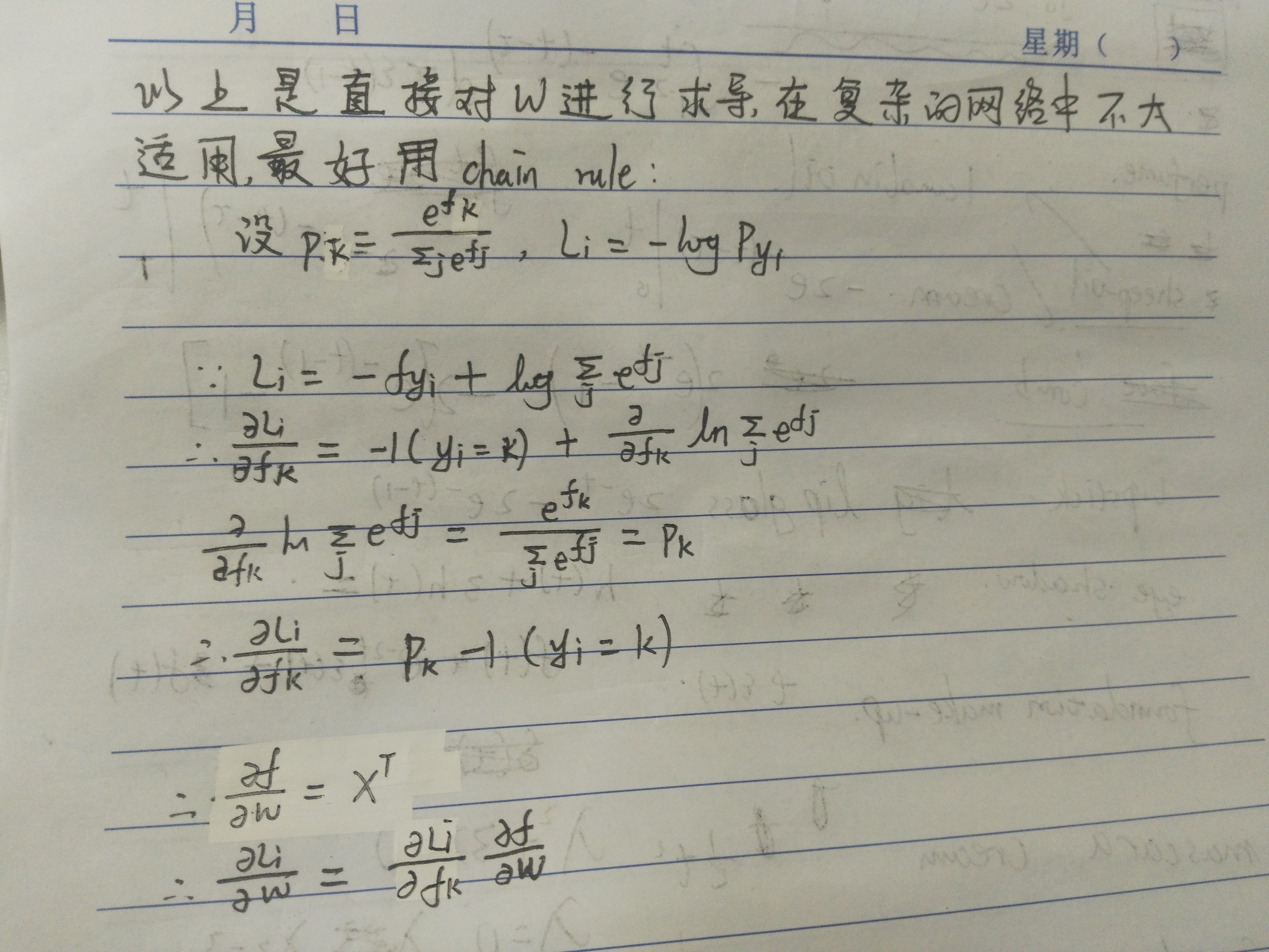
难点在于dW的求解

此处参考了https://www.jianshu.com/p/6e405cecd609 ，我修改了一下原作中一些不太清晰的下标

b.softmax_loss_vectorized代码实现和推导

代码：

def softmax_loss_vectorized(W, X, y, reg):
  """
  Softmax loss function, vectorized version.

  Inputs and outputs are the same as softmax_loss_naive.
  """
  # Initialize the loss and gradient to zero.
  loss = 0.0
  dW = np.zeros_like(W)

  #############################################################################
  # TODO: Compute the softmax loss and its gradient using no explicit loops.  #
  # Store the loss in loss and the gradient in dW. If you are not careful     #
  # here, it is easy to run into numeric instability. Don't forget the        #
  # regularization!                                                           #
  #############################################################################
  num_train = X.shape[0]
  num_classes = W.shape[1]
  scores = X.dot(W)
  scores_row_max = np.max(scores, axis=1).reshape(-1,1)
  scores -= scores_row_max

  correct_class_scores = scores[np.arange(num_train), y]

  loss += -np.sum(correct_class_scores) + np.sum(np.log(np.sum(np.exp(scores),axis=1)))
  loss /= num_train
  loss += reg*np.sum(W*W)

  Pj = np.exp(scores)/(np.sum(np.exp(scores), axis=1).reshape(-1,1))
  Pj[range(num_train), y] -= 1
  dW = X.T.dot(Pj)
  dW /= num_train
  dW += reg*W
  #############################################################################
  #                          END OF YOUR CODE                                 #
  #############################################################################

  return loss, dW

代码解析：

loss函数的实现相对简单，dW的矩阵化计算较为巧妙，实现公式

 if  j==yi 则 dW = X*(Pj -1)

     j!=yi 则 dW = X*Pj

其中Pj为                                                 

2.softmax.ipynb

用validation调整参数部分代码

# Use the validation set to tune hyperparameters (regularization strength and
# learning rate). You should experiment with different ranges for the learning
# rates and regularization strengths; if you are careful you should be able to
# get a classification accuracy of over 0.35 on the validation set.
from cs231n.classifiers import Softmax
results = {}
best_val = -1
best_softmax = None
learning_rates = [5e-7,5.5e7, 6e-7]
regularization_strengths = [5e4, 5.5e4]


################################################################################
# TODO:                                                                        #
# Use the validation set to set the learning rate and regularization strength. #
# This should be identical to the validation that you did for the SVM; save    #
# the best trained softmax classifer in best_softmax.                          #
################################################################################
Softmax = Softmax()
iters = 500
for lr in learning_rates:
    for rs in regularization_strengths:
        Softmax.train(X_train, y_train, learning_rate=lr, reg=rs, num_iters=iters)
        y_train_pred = Softmax.predict(X_train)
        accu_train = np.mean(y_train==y_train_pred)
        y_val_pred = Softmax.predict(X_val)
        accu_val = np.mean(y_val==y_val_pred)
        results[(lr,rs)] = (accu_train, accu_val)
        if best_val < accu_val:
            best_softmax = Softmax
            best_val = accu_val
################################################################################
#                              END OF YOUR CODE                                #
################################################################################
    
# Print out results.
for lr, reg in sorted(results):
    train_accuracy, val_accuracy = results[(lr, reg)]
    print('lr %e reg %e train accuracy: %f val accuracy: %f' % (
                lr, reg, train_accuracy, val_accuracy))
    
print('best validation accuracy achieved during cross-validation: %f' % best_val)

此处和svm的一样，记得第一行要进行Sotfmax类的实例化

四、Two_layer_net

1.neutral_net.py

a.loss函数实现和推导

代码：

  def loss(self, X, y=None, reg=0.0):
    """
    Compute the loss and gradients for a two layer fully connected neural
    network.

    Inputs:
    - X: Input data of shape (N, D). Each X[i] is a training sample.
    - y: Vector of training labels. y[i] is the label for X[i], and each y[i] is
      an integer in the range 0 <= y[i] < C. This parameter is optional; if it
      is not passed then we only return scores, and if it is passed then we
      instead return the loss and gradients.
    - reg: Regularization strength.

    Returns:
    If y is None, return a matrix scores of shape (N, C) where scores[i, c] is
    the score for class c on input X[i].

    If y is not None, instead return a tuple of:
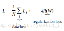
    - loss: Loss (data loss and regularization loss) for this batch of training
      samples.
    - grads: Dictionary mapping parameter names to gradients of those parameters
      with respect to the loss function; has the same keys as self.params.
    """
    # Unpack variables from the params dictionary
    W1, b1 = self.params['W1'], self.params['b1']
    W2, b2 = self.params['W2'], self.params['b2']
    N, D = X.shape

    # Compute the forward pass
    scores = None
    #############################################################################
    # TODO: Perform the forward pass, computing the class scores for the input. #
    # Store the result in the scores variable, which should be an array of      #
    # shape (N, C).                                                             #
    #############################################################################
    f = lambda x: np.maximum(0,x)
    # f = lambda x: np.tanh(x)
    # f = lambda x: 1/(1+np.exp(x))
    a1 = np.dot(X,W1) + b1
    h1 = f(a1)
    a2 = np.dot(h1,W2) + b2
    scores = a2
    #############################################################################
    #                              END OF YOUR CODE                             #
    #############################################################################
    
    # If the targets are not given then jump out, we're done
    if y is None:
      return scores

    # Compute the loss
    loss = None
    #############################################################################
    # TODO: Finish the forward pass, and compute the loss. This should include  #
    # both the data loss and L2 regularization for W1 and W2. Store the result  #
    # in the variable loss, which should be a scalar. Use the Softmax           #
    # classifier loss.                                                          #
    #############################################################################
    scores_row_max = np.max(scores, axis=1).reshape(-1,1)
    scores -= scores_row_max
    correct_class_scores = scores[np.arange(N), y]
    loss = -np.sum(correct_class_scores) + np.sum(np.log(np.sum(np.exp(scores), axis=1)))
    loss /= N
    loss += reg * (np.sum(W1 * W1)+np.sum(W2*W2))
    #############################################################################
    #                              END OF YOUR CODE                             #
    #############################################################################

    # Backward pass: compute gradients
    grads = {}
    #############################################################################
    # TODO: Compute the backward pass, computing the derivatives of the weights #
    # and biases. Store the results in the grads dictionary. For example,       #
    # grads['W1'] should store the gradient on W1, and be a matrix of same size #
    #############################################################################
    P = np.exp(scores) / (np.sum(np.exp(scores), axis=1).reshape(-1, 1))
    dscores = P
    dscores[range(N),y] -= 1
    dscores /= N
    dW2 = np.dot(h1.T, dscores) + 2*reg*W2
    db2 = np.sum(dscores, axis=0, keepdims=False)
    da2 = np.dot(dscores,W2.T)
    da2[a1 < 0] = 0
    dW1 = np.dot(X.T,da2) + 2*reg*W1
    db1 = np.sum(da2, axis=0, keepdims=False)
    grads['W1'] = dW1
    grads['b1'] = db1
    grads['W2'] = dW2
    grads['b2'] = db2

    #############################################################################
    #                              END OF YOUR CODE                             #
    #############################################################################

    return loss, grads

par1. forward pass

    # Compute the forward pass
    scores = None
    #############################################################################
    # TODO: Perform the forward pass, computing the class scores for the input. #
    # Store the result in the scores variable, which should be an array of      #
    # shape (N, C).                                                             #
    #############################################################################
    f = lambda x: np.maximum(0,x)
    # f = lambda x: np.tanh(x)
    # f = lambda x: 1/(1+np.exp(x))
    a1 = np.dot(X,W1) + b1
    h1 = f(a1)
    a2 = np.dot(h1,W2) + b2
    scores = a2
    #############################################################################
    #                              END OF YOUR CODE                             #
    #############################################################################
    
    # If the targets are not given then jump out, we're done
    if y is None:
      return scores

代码解释：

用Relu激活函数，注释掉的两行是用了logsitic函数和tanh函数试了，效果远不如Relu函数的好，剩下的就是前向传播计算

part2. loss

    # Compute the loss
    loss = None
    #############################################################################
    # TODO: Finish the forward pass, and compute the loss. This should include  #
    # both the data loss and L2 regularization for W1 and W2. Store the result  #
    # in the variable loss, which should be a scalar. Use the Softmax           #
    # classifier loss.                                                          #
    #############################################################################
    scores_row_max = np.max(scores, axis=1).reshape(-1,1)
    scores -= scores_row_max
    correct_class_scores = scores[np.arange(N), y]
    loss = -np.sum(correct_class_scores) + np.sum(np.log(np.sum(np.exp(scores), axis=1)))
    loss /= N
    loss += reg * (np.sum(W1 * W1)+np.sum(W2*W2))
    #############################################################################
    #                              END OF YOUR CODE                             #
    #############################################################################

代码解释：

先将scores归一化，然后计算使用了softmax分类器后的loss function

part3. Backward pass: compute gradients

    # Backward pass: compute gradients
    grads = {}
    #############################################################################
    # TODO: Compute the backward pass, computing the derivatives of the weights #
    # and biases. Store the results in the grads dictionary. For example,       #
    # grads['W1'] should store the gradient on W1, and be a matrix of same size #
    #############################################################################
    P = np.exp(scores) / (np.sum(np.exp(scores), axis=1).reshape(-1, 1))
    dscores = P
    dscores[range(N),y] -= 1
    dscores /= N
    dW2 = np.dot(h1.T, dscores) + 2*reg*W2
    db2 = np.sum(dscores, axis=0, keepdims=False)
    da2 = np.dot(dscores,W2.T)
    da2[a1 < 0] = 0
    dW1 = np.dot(X.T,da2) + 2*reg*W1
    db1 = np.sum(da2, axis=0, keepdims=False)
    grads['W1'] = dW1
    grads['b1'] = db1
    grads['W2'] = dW2
    grads['b2'] = db2

    #############################################################################
    #                              END OF YOUR CODE                             #
    #############################################################################

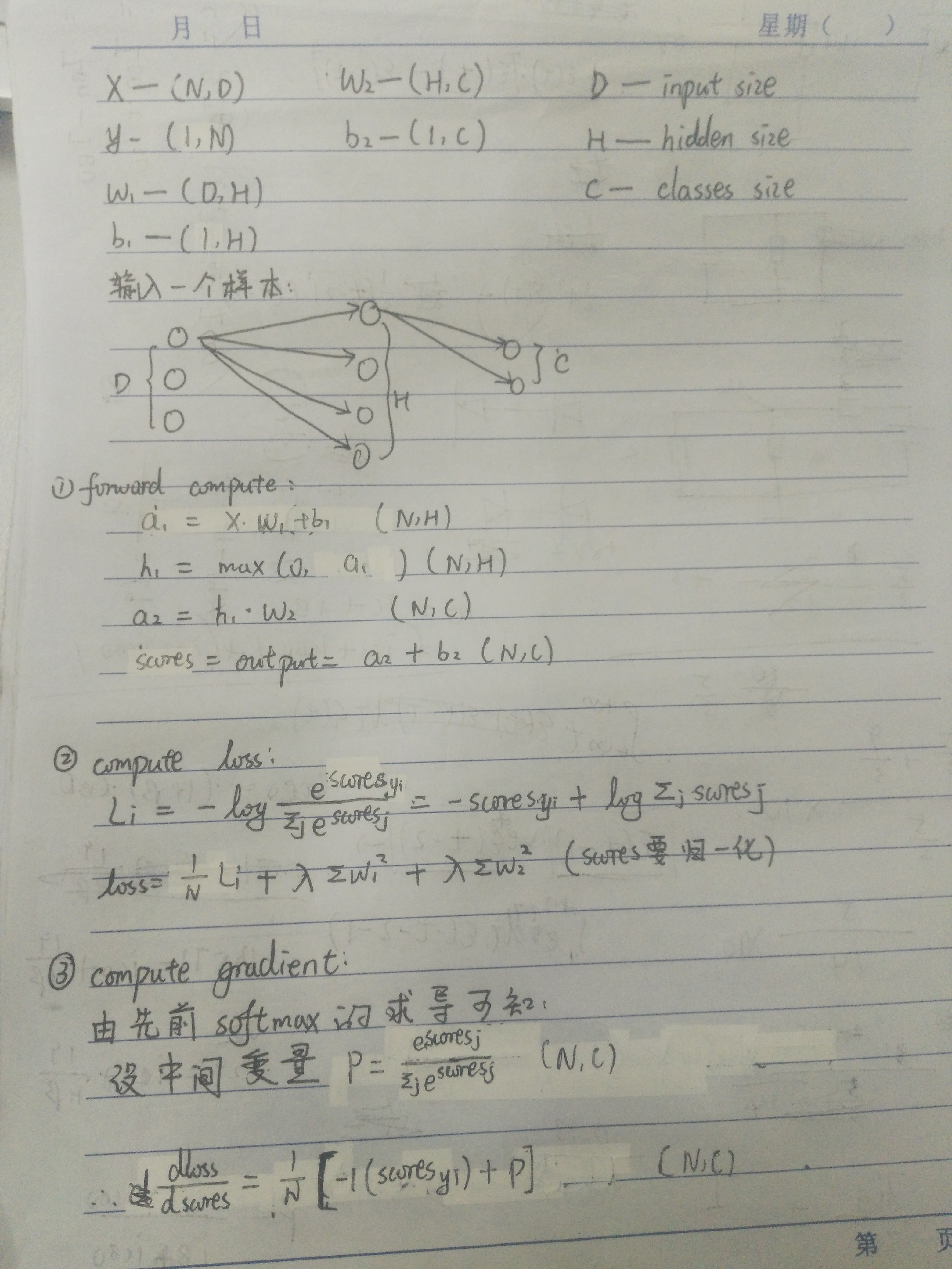
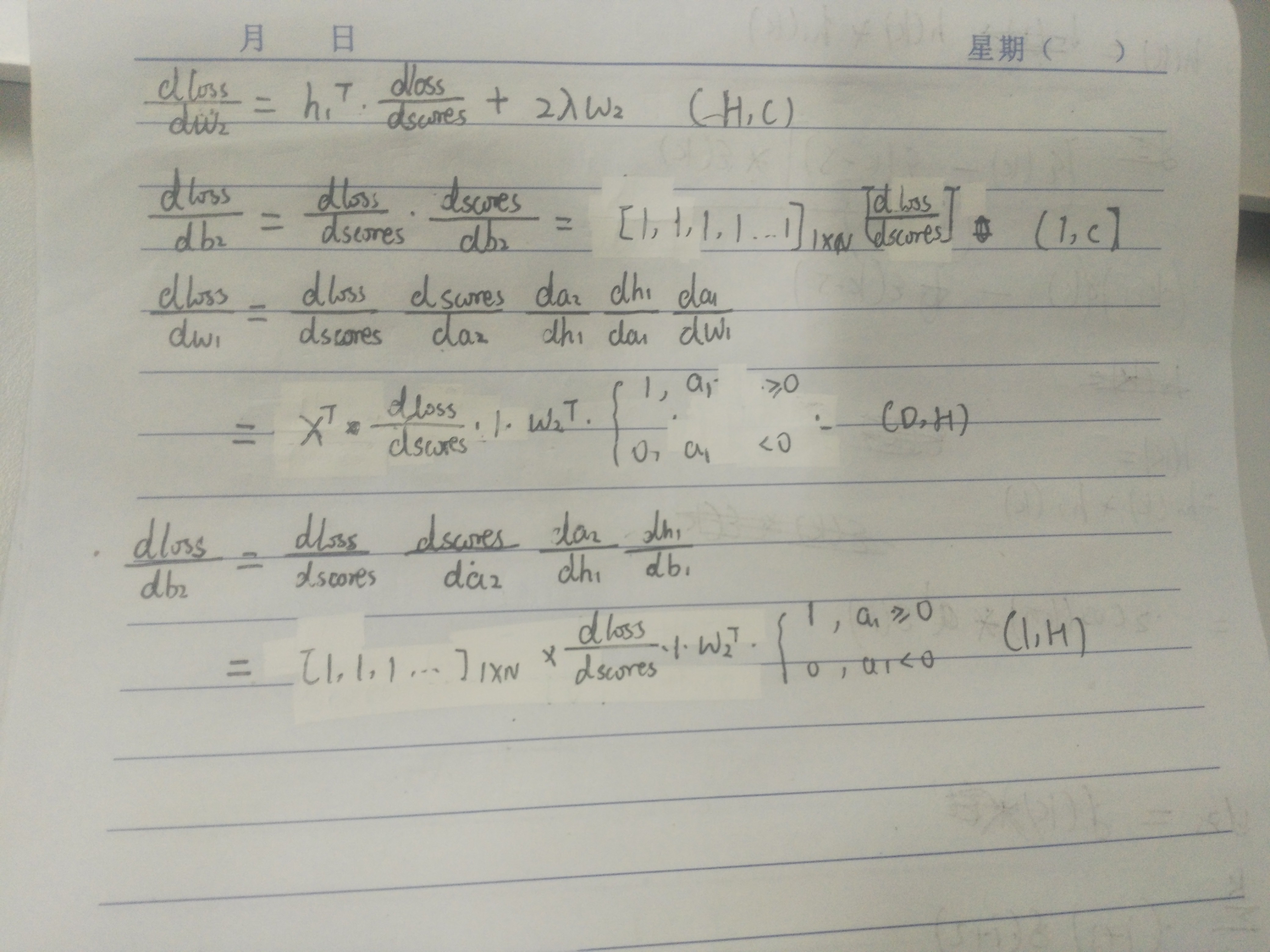
    return loss, grads

梯度推导：

part4. train（use SGD)

  def train(self, X, y, X_val, y_val,
            learning_rate=1e-3, learning_rate_decay=0.95,
            reg=5e-6, num_iters=100,
            batch_size=200, verbose=False):
    """
    Train this neural network using stochastic gradient descent.

    Inputs:
    - X: A numpy array of shape (N, D) giving training data.
    - y: A numpy array f shape (N,) giving training labels; y[i] = c means that
      X[i] has label c, where 0 <= c < C.
    - X_val: A numpy array of shape (N_val, D) giving validation data.
    - y_val: A numpy array of shape (N_val,) giving validation labels.
    - learning_rate: Scalar giving learning rate for optimization.
    - learning_rate_decay: Scalar giving factor used to decay the learning rate
      after each epoch.
    - reg: Scalar giving regularization strength.
    - num_iters: Number of steps to take when optimizing.
    - batch_size: Number of training examples to use per step.
    - verbose: boolean; if true print progress during optimization.
    """
    num_train = X.shape[0]
    iterations_per_epoch = max(num_train / batch_size, 1)

    # Use SGD to optimize the parameters in self.model
    loss_history = []
    train_acc_history = []
    val_acc_history = []

    for it in xrange(num_iters):
      X_batch = None
      y_batch = None

      #########################################################################
      # TODO: Create a random minibatch of training data and labels, storing  #
      # them in X_batch and y_batch respectively.                             #
      #########################################################################
      sample_index = np.random.choice(num_train,batch_size)
      X_batch = X[sample_index]
      y_batch = y[sample_index]
      #########################################################################
      #                             END OF YOUR CODE                          #
      #########################################################################

      # Compute loss and gradients using the current minibatch
      loss, grads = self.loss(X_batch, y=y_batch, reg=reg)
      loss_history.append(loss)

      #########################################################################
      # TODO: Use the gradients in the grads dictionary to update the         #
      # parameters of the network (stored in the dictionary self.params)      #
      # using stochastic gradient descent. You'll need to use the gradients   #
      # stored in the grads dictionary defined above.                         #
      #########################################################################
      self.params['W1'] -= learning_rate*grads['W1']
      self.params['b1'] -= learning_rate*grads['b1']
      self.params['W2'] -= learning_rate*grads['W2']
      self.params['b2'] -= learning_rate*grads['b2']
      #########################################################################
      #                             END OF YOUR CODE                          #
      #########################################################################

      if verbose and it % 100 == 0:
        print('iteration %d / %d: loss %f' % (it, num_iters, loss))

      # Every epoch, check train and val accuracy and decay learning rate.
      if it % iterations_per_epoch == 0:
        # Check accuracy
        train_acc = (self.predict(X_batch) == y_batch).mean()
        val_acc = (self.predict(X_val) == y_val).mean()
        train_acc_history.append(train_acc)
        val_acc_history.append(val_acc)

        # Decay learning rate
        learning_rate *= learning_rate_decay

    return {
      'loss_history': loss_history,
      'train_acc_history': train_acc_history,
      'val_acc_history': val_acc_history,
    }

类似前面的linear_classifier中的代码，相对简单

part6.predict

  def predict(self, X):
    """
    Use the trained weights of this two-layer network to predict labels for
    data points. For each data point we predict scores for each of the C
    classes, and assign each data point to the class with the highest score.

    Inputs:
    - X: A numpy array of shape (N, D) giving N D-dimensional data points to
      classify.

    Returns:
    - y_pred: A numpy array of shape (N,) giving predicted labels for each of
      the elements of X. For all i, y_pred[i] = c means that X[i] is predicted
      to have class c, where 0 <= c < C.
    """
    y_pred = None

    ###########################################################################
    # TODO: Implement this function; it should be VERY simple!                #
    ###########################################################################
    f = lambda x: np.maximum(0, x)
    a1 = np.dot(X, self.params['W1']) + self.params['b1']
    h1 = f(a1)
    a2 = np.dot(h1, self.params['W2']) + self.params['b2']
    scores = a2
    y_pred = np.argmax(scores,axis=1)
    ###########################################################################
    #                              END OF YOUR CODE                           #
    ###########################################################################

    return y_pred

用更新的值去计算最后的类别