[CS231n Assignment #1] 简单图像分类器——SVM线性分类器

文章目录

作业介绍
知识点简单回顾
1. 下载数据集
2. SVM分类器

2.1 预处理与显示
2.2 完成SVM分类器

作业提问
参考资料

作业介绍

作业主页：Assignment #1
作业目的：
- 针对SVM，实现一个全向量化的 损失函数(loss function)
- 实现损失函数的矢量化解析梯度（analytic gradient）
- 用 数值梯度（numerical gradient） 检验解析梯度是否正确
- 使用测试集（val set）调试学习率和正则化程度大小（ the learning rate and regularization）
- 使用 SGD 更新策略最优化我们的SVM损失函数
- 可视化最后学习到的权重
官方给的示例代码：assigment #1 code

知识点简单回顾

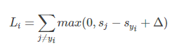
多类支持向量机（Support Vector Machine, SVM）的分类目标是使得正确类别的得分（ $W^TX$ ）比其它类别的得分尽可能的大一个间隔(margin)，用 $\bigtriangleup$ 来表示。
对于单个样本 $x_i$ ，其损失函数表示为：
在这里插入图片描述
将 $s_j = W^T_j * x_i, s_{y_i} = W^T_{y_i}*x_i$ （即第 $j$ 类的得分和第 $y_i$ 类别的得分）带入上式有：

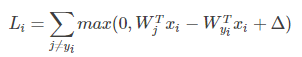
其中， $(x_i,y_i)$ 表示正确类别， $s_{y_i}$ 表示正确类别预测的分数， $s_j$ 表示错误类别预测的分数。即我们希望 $s_j$ 比 $s_{y_i}$ 要小 $\bigtriangleup$ 。

在这里插入图片描述
所以该损失也被称为合页损失（Hinge Loss）。

举个例子，对于CIFAR 10，输入的X的维度是[1,3072]，而W的维度是[3072,10]，所以 $W_j$ 表示第 $j$ 列，也就是第 $j$ 个分类模板， $X*W$ 的维度是 [1,10] 有10个类别的得分。

同时为了防止过拟合，我们引入正则项：
在这里插入图片描述

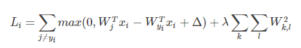
L2范数正则项限制权重W过大，使其更小且分布均匀。而L1正则项使得W分布得更稀疏，更离散。

1. 下载数据集

参照之前的 KNN 分类器

2. SVM分类器

使用 jupyter nodetebook 打开文件 svm.ipynb 梳理一下流程（期间没有的python库需要自己手动安装一下）

2.1 预处理与显示

只是需要注意以下几点：

图像减去均值的时候是 逐像素(element-wise) 减去该位置像素值在训练集的均值

# Preprocessing: subtract the mean image
# first: compute the image mean based on the training data
mean_image = np.mean(X_train, axis=0)
print(mean_image[:10]) # print a few of the elements
plt.figure(figsize=(4,4))
plt.imshow(mean_image.reshape((32,32,3)).astype('uint8')) # visualize the mean image
plt.show()

# second: subtract the mean image from train and test data
X_train -= mean_image
X_val -= mean_image
X_test -= mean_image
X_dev -= mean_image

# third: append the bias dimension of ones (i.e. bias trick) so that our SVM
# only has to worry about optimizing a single weight matrix W.
X_train = np.hstack([X_train, np.ones((X_train.shape[0], 1))])
X_val = np.hstack([X_val, np.ones((X_val.shape[0], 1))])
X_test = np.hstack([X_test, np.ones((X_test.shape[0], 1))])
X_dev = np.hstack([X_dev, np.ones((X_dev.shape[0], 1))])

print(X_train.shape, X_val.shape, X_test.shape, X_dev.shape)
# (49000L, 3073L) (1000L, 3073L) (1000L, 3073L) (500L, 3073L)

并且需要给每个样本 $X_i(1,3072)$ 添加一个维度变成 (1,3073) 这样我们就不用显示的表示偏置项 $b$ ，而只需要将权重矩阵对应的增加为 $(3073,10)$ 即可。

2.2 完成SVM分类器

完成在cs231n/classifiers/linear_svm.py中的填充代码并测试。

1. 实现矢量化的损失函数

循环版本

def svm_loss_naive(W, X, y, reg):
  """
  Inputs:
  - W: A numpy array of shape (D, C) containing weights.
  - X: A numpy array of shape (N, D) containing a minibatch of data.
  - y: A numpy array of shape (N,) containing training labels; y[i] = c means
    that X[i] has label c, where 0 <= c < C.
  - reg: (float) regularization strength

  Returns a tuple of:
  - loss as single float
  - gradient with respect to weights W; an array of same shape as W
  """
  dW = np.zeros(W.shape) # initialize the gradient as zero

  # compute the loss and the gradient
  num_classes = W.shape[1]
  num_train = X.shape[0]
  loss = 0.0
  for i in range(num_train):
    scores = X[i].dot(W)
    correct_class_score = scores[y[i]]
    for j in range(num_classes):
      if j == y[i]:
        continue
      margin = scores[j] - correct_class_score + 1 # note delta = 1
      if margin > 0:
        loss += margin
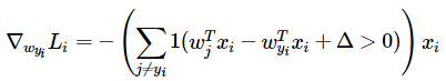
        # 代表了我们应该增大正确分类的权重，减少错误分类的权重
        dW[:,j] += X[i].T
        dW[:,y[i]] -= X[i].T
  # Right now the loss is a sum over all training examples, but we want it
  # to be an average instead so we divide by num_train.
  loss /= num_train
  dW /= num_train
  # Add regularization to the loss.
  # 乘以 0.5 这样我们在求dW的时候就没有系数了
  loss += 0.5 * reg * np.sum(W * W)
  dW += reg * W
  return loss, dW

# Evaluate the naive implementation of the loss we provided for you:
from cs231n.classifiers.linear_svm import svm_loss_naive
import time

# generate a random SVM weight matrix of small numbers
W = np.random.randn(3073, 10) * 0.0001 

loss, grad = svm_loss_naive(W, X_dev, y_dev, 0.000005)
print('loss: %f' % (loss, ))
# loss: 8.949549

向量化版本

def svm_loss_vectorized(W, X, y, reg):
  """
  Structured SVM loss function, vectorized implementation.
  Inputs:
  - W: A numpy array of shape (D, C) containing weights.
  - X: A numpy array of shape (N, D) containing a minibatch of data.
  - y: A numpy array of shape (N,) containing training labels; y[i] = c means
    that X[i] has label c, where 0 <= c < C.
  - reg: (float) regularization strength

  Returns a tuple of:
  - loss as single float
  - gradient with respect to weights W; an array of same shape as W
  """
  loss = 0.0
  dW = np.zeros(W.shape) # initialize the gradient as zero
  num_train = X.shape[0]
  # 计算损失
  # (1) 先算出得分矩阵
  scores = X.dot(W) # [N , C]
  # (2) 再抽离出每个类别正确分类的得分
  # 使用数组索引取出每行的正确得分
  scores_yi = scores[range(num_train),y].reshape(-1,1) # [N , 1]
  # (3)利用广播机制进行相减
  scores_sub = scores - scores_yi + 1.0 # 注意margin
  # Attention!!! 这里需要将正确分类加的 margin 去掉
  scores_sub[range(num_train),list(y)] = 0
  # 略去非正数部分
  scores_sub = np.maximum(0,scores_sub)
  loss = np.sum(scores_sub) / num_train + 0.5 * reg * np.sum(W * W) # 加上二范数

  # 计算梯度
  # (1) 先找到我们最后计算的损失里面每一列中不为0的部分
  # 其代表与当前列相关的权重有关的样本索引
  num_classes = W.shape[1]
  mask = np.zeros((num_train,num_classes))
  mask[scores_sub > 0] = 1 # 挑出有关样本
  # 计算正样本的反传
  mask[range(num_train),list(y)] = 0
  mask[range(num_train),list(y)] -= np.sum(mask,axis = 1) # 每一个负样本都会更新该权重
  dW = np.dot(X.T,mask) # [N , C]
  dW = dW / num_train + reg * W
  return loss, dW

梯度检验

# Compute the loss and its gradient at W.
loss, grad = svm_loss_naive(W, X_dev, y_dev, 0.0)

# Numerically compute the gradient along several randomly chosen dimensions, and
# compare them with your analytically computed gradient. The numbers should match
# almost exactly along all dimensions.
from cs231n.gradient_check import grad_check_sparse
f = lambda w: svm_loss_naive(w, X_dev, y_dev, 0.0)[0] # 输入w返回损失loss
grad_numerical = grad_check_sparse(f, W, grad)

# do the gradient check once again with regularization turned on
# you didn't forget the regularization gradient did you?
loss, grad = svm_loss_naive(W, X_dev, y_dev, 5e1)
f = lambda w: svm_loss_naive(w, X_dev, y_dev, 5e1)[0]
grad_numerical = grad_check_sparse(f, W, grad)

检验原理
损失函数 L 对权值 W 的梯度是和 W相同维度的，根据梯度的定义，我们可以选择 W 中的某一位置，然后稍微增大一点后，再次计算损失，然后计算变化程度，就是损失对该位置的偏导数。

def grad_check_sparse(f, x, analytic_grad, num_checks=10, h=1e-5):
  """
  sample a few random elements and only return numerical
  in this dimensions.
  """
  for i in range(num_checks):
    # 在 x 的每一个维度都随机选择一个索引位置求数值梯度
    ix = tuple([randrange(m) for m in x.shape])

    oldval = x[ix]
    x[ix] = oldval + h # increment by h
    fxph = f(x) # evaluate f(x + h)
    x[ix] = oldval - h # increment by h
    fxmh = f(x) # evaluate f(x - h)
    x[ix] = oldval # reset

    grad_numerical = (fxph - fxmh) / (2 * h)
    grad_analytic = analytic_grad[ix]
    rel_error = abs(grad_numerical - grad_analytic) / (abs(grad_numerical) + abs(grad_analytic))
    print('numerical: %f analytic: %f, relative error: %e' % (grad_numerical, grad_analytic, rel_error))

时间和正确性比较

平时为了防止代码有错，我们也可以先写一个比较笨的算法，再写一个高效的算法，进行结果的比较

import time
tic = time.time()
loss_naive, grad_naive = svm_loss_naive(W, X_dev, y_dev, 0.000005)
toc = time.time()
print('Naive loss: %e computed in %fs' % (loss_naive, toc - tic))

from cs231n.classifiers.linear_svm import svm_loss_vectorized
tic = time.time()
loss_vectorized, _ = svm_loss_vectorized(W, X_dev, y_dev, 0.000005)
toc = time.time()
print('Vectorized loss: %e computed in %fs' % (loss_vectorized, toc - tic))

# The losses should match but your vectorized implementation should be much faster.
print('difference: %f' % (loss_naive - loss_vectorized))

tic = time.time()
_, grad_naive = svm_loss_naive(W, X_dev, y_dev, 0.000005)
toc = time.time()
print('Naive loss and gradient: computed in %fs' % (toc - tic))

tic = time.time()
_, grad_vectorized = svm_loss_vectorized(W, X_dev, y_dev, 0.000005)
toc = time.time()
print('Vectorized loss and gradient: computed in %fs' % (toc - tic))

# The loss is a single number, so it is easy to compare the values computed
# by the two implementations. The gradient on the other hand is a matrix, so
# we use the Frobenius norm to compare them.
difference = np.linalg.norm(grad_naive - grad_vectorized, ord='fro')
print('difference: %f' % difference)

2. 随机梯度下降（SGD）更新参数

首先实现cs231n\classifiers\linear_classifier.py中的线性分类器LinearClassifier和SVM分类部分。

class LinearClassifier(object):

    def __init__(self):
        self.W = None

    def train(self, X, y, learning_rate=1e-3, reg=1e-5, num_iters=100,
              batch_size=200, verbose=False):
        """
        Train this linear classifier using stochastic gradient descent.

        Inputs:
        - X: A numpy array of shape (N, D) containing training data; there are N
          training samples each of dimension D.
        - y: A numpy array of shape (N,) containing training labels; y[i] = c
          means that X[i] has label 0 <= c < C for C classes.
        - learning_rate: (float) learning rate for optimization.
        - reg: (float) regularization strength.
        - num_iters: (integer) number of steps to take when optimizing
        - batch_size: (integer) number of training examples to use at each step.
        - verbose: (boolean) If true, print progress during optimization.

        Outputs:
        A list containing the value of the loss function at each training iteration.
        """
        num_train, dim = X.shape
        num_classes = np.max(y) + 1 # assume y takes values 0...K-1 where K is number of classes
        if self.W is None:
            # lazily initialize W
            self.W = 0.001 * np.random.randn(dim, num_classes)

        # Run stochastic gradient descent to optimize W
        loss_history = []
        for it in range(num_iters):
            X_batch = None
            y_batch = None

            # 从 0 ~ num_train - 1 中随机选择 batch_size 个数
            # 问题不能讲样本取尽
            batch_indices = np.random.choice(num_train,batch_size,replace = True)
            X_batch = X[batch_indices]
            y_batch = y[batch_indices]

            # evaluate loss and gradient
            loss, grad = self.loss(X_batch, y_batch, reg)
            loss_history.append(loss)

            # Update the weights using the gradient and the learning rate.          #
            self.W -= learning_rate * grad

            if verbose and it % 100 == 0:
                print('iteration %d / %d: loss %f' % (it, num_iters, loss))

        return loss_history

# 训练测试代码
# In the file linear_classifier.py, implement SGD in the function
# LinearClassifier.train() and then run it with the code below.
from cs231n.classifiers import LinearSVM
svm = LinearSVM()
tic = time.time()
loss_hist = svm.train(X_train, y_train, learning_rate=1e-7, reg=2.5e4,
                      num_iters=1500, verbose=True)
toc = time.time()
print('That took %fs' % (toc - tic))

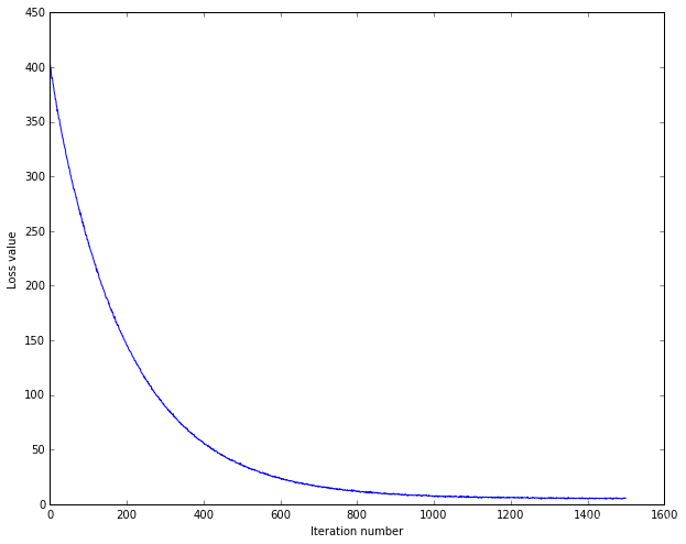
# 画出每次迭代的损失图
plt.plot(loss_hist)
plt.xlabel('Iteration number')
plt.ylabel('Loss value')
plt.show()

在这里插入图片描述
3. 完成预测阶段

接收测试图像
对于每个图像，输出C类得分
取出得分最大的类别作为其标签

 def predict(self, X):
        """
        Use the trained weights of this linear classifier to predict labels for
        data points.

        Inputs:
        - X: A numpy array of shape (N, D) containing training data; there are N
          training samples each of dimension D.

        Returns:
        - y_pred: Predicted labels for the data in X. y_pred is a 1-dimensional
          array of length N, and each element is an integer giving the predicted
          class.
        """
        y_pred = np.zeros(X.shape[0])
        scores = np.dot(X,self.W)
        y_pred = np.argmax(scores,axis = 1) # 取出每一行最大得分类别
        return y_pred

# Write the LinearSVM.predict function and evaluate the performance on both the
# training and validation set
y_train_pred = svm.predict(X_train)
print('training accuracy: %f' % (np.mean(y_train == y_train_pred), ))
y_val_pred = svm.predict(X_val)
print('validation accuracy: %f' % (np.mean(y_val == y_val_pred), ))

training accuracy: 0.381673
validation accuracy: 0.393000

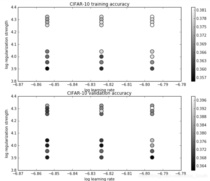
4. 使用验证集(validation)和测试集调参

设置参数，例如学习率和正则化强度的变化范围
参数在指定范围内变化，然后计算其在验证集上的精度
选择多次验证后的最优参数，然后计算其在测试集上的性能

# Use the validation set to tune hyperparameters (regularization strength and
# learning rate).
learning_rates = [1.4e-7, 1.5e-7, 1.6e-7]
regularization_strengths = [8000.0, 9000.0, 10000.0, 11000.0, 18000.0, 19000.0, 20000.0, 21000.0]

# results is dictionary mapping tuples of the form
# (learning_rate, regularization_strength) to tuples of the form
# (training_accuracy, validation_accuracy). 
results = {}
best_lr = None
best_reg = None
best_val = -1   # The highest validation accuracy that we have seen so far.
best_svm = None # The LinearSVM object that achieved the highest validation rate.
                                                                           
# Hint: You should use a small value for num_iters as you develop your         #
# validation code so that the SVMs don't take much time to train; once you are #
# confident that your validation code works, you should rerun the validation   #
# code with a larger value for num_iters.                                      #

num_iters = 800 # 先使用小的迭代次数验证代码能否正常运行
for lr in learning_rates:
    for rs in regularization_strengths:
        svm = LinearSVM()
        train_loss = svm.train(X_train,y_train,lr,rs,num_iters)
        y_train_pred = svm.predict(X_train)
        y_train_acc = np.mean(y_train_pred == y_train)
        y_val_pred = svm.predict(X_val)
        y_val_acc = np.mean(y_val_pred == y_val)
        results[(lr,rs)] = (y_train_acc,y_val_acc)
        if y_val_acc > best_val:
            best_val = y_val_acc
            best_svm = svm
            best_lr = lr
            best_reg = rs
  
# Print out results.
for lr, reg in sorted(results):
    train_accuracy, val_accuracy = results[(lr, reg)]
    print('lr %e reg %e train accuracy: %f val accuracy: %f' % (
                lr, reg, train_accuracy, val_accuracy))
    
print('Best validation accuracy during cross-validation:\nlr = %e, reg = %e, best_val = %f' %
      (best_lr, best_reg, best_val))

可视化每组参数对应的准确度：

import math
x_scatter = [math.log10(x[0]) for x in results]
y_scatter = [math.log10(x[1]) for x in results]

# plot training accuracy
marker_size = 100
colors = [results[x][0] for x in results]
plt.subplot(2, 1, 1)
plt.scatter(x_scatter, y_scatter, marker_size, c=colors)
plt.colorbar()
plt.xlabel('log learning rate')
plt.ylabel('log regularization strength')
plt.title('CIFAR-10 training accuracy')

# plot validation accuracy
colors = [results[x][1] for x in results] # default size of markers is 20
plt.subplot(2, 1, 2)
plt.scatter(x_scatter, y_scatter, marker_size, c=colors)
plt.colorbar()
plt.xlabel('log learning rate')
plt.ylabel('log regularization strength')
plt.title('CIFAR-10 validation accuracy')
plt.show()

在这里插入图片描述
选择最好的参数在测试集(test)上测试性能：

y_test_pred = best_svm.predict(X_test)
test_accuracy = np.mean(y_test == y_test_pred)
print('linear SVM on raw pixels final test set accuracy: %f' % test_accuracy)

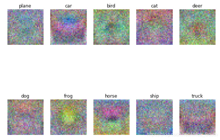
5. 可视化学习到的权重

对于每个类别，权重模板的维度是 $1*3072$ , 我们可以将其还原成维度为 $32*32*3$ ，然后显示成RGB图像
注意需要标准化到 [0,255]

w = best_svm.W[:-1,:] # strip out the bias
w = w.reshape(32, 32, 3, 10)
w_min, w_max = np.min(w), np.max(w)
classes = ['plane', 'car', 'bird', 'cat', 'deer', 'dog', 'frog', 'horse', 'ship', 'truck']
for i in range(10):
    plt.subplot(2, 5, i + 1)
      
    # Rescale the weights to be between 0 and 255
    # 这里抽掉了最后一维
    wimg = 255.0 * (w[:, :, :, i].squeeze() - w_min) / (w_max - w_min)
    plt.imshow(wimg.astype('uint8'))
    plt.axis('off')
    plt.title(classes[i])

在这里插入图片描述

作业提问

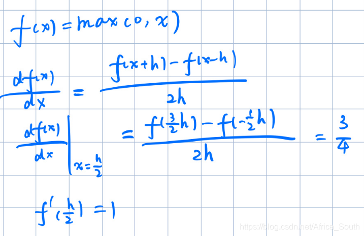
Q1:It is possible that once in a while a dimension in the gradcheck will not match exactly. What could such a discrepancy be caused by? Is it a reason for concern? What is a simple example in one dimension where a gradient check could fail? How would change the margin affect of the frequency of this happening? Hint: the SVM loss function is not strictly speaking differentiable
A1: 原因可能是最大值函数 $f(x) = max(0,x)$ 在 $x = 0$ 处是连续但是不可微的，从图像上来看
-
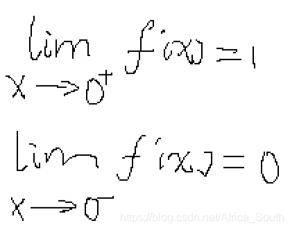
所以可能出现在0附近解析梯度与数值梯度不一致的情况。例如：
Q2： Describe what your visualized SVM weights look like, and offer a brief explanation for why they look they way that they do.
A2： 学习到的权重是 $W^{D*C}$ ，每一列到表示一类的模板，将其可视化后优点类似于该类图像的一个均值图。因为，按照我们的损失函数来看，该类模板与该类图像的得分结果应该比其它模板大，也就是它们的乘积值越大，而如果考虑两个单位向量的余弦距离，则两个单位向量越是同方向，也就是该类模板与该类图像越接近，则它们的乘积越大。