任务:
- 完成一个基于SVM的全向量化损失函数
- 完成解析梯度的全向量化表示
- 用数值梯度来验证
- 使用一个验证集去调优 learning rate 和 regularization
- 使用SGD方法
- 可视化最优的Weight
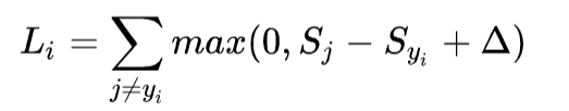
SVM的 loss function 为:
- 首先,加载原始数据并做简单的数据划分
import random
import numpy as np
from cs231n.data_utils import load_CIFAR10
import matplotlib.pyplot as plt
from cs231n.classifiers.linear_svm import svm_loss_naive
from cs231n.gradient_check import grad_check_sparse
import time

cifar10_dir = 'F:\pycharmFile\KNN\cifar-10-batches-py'
X_train, y_train, X_test, y_test = load_CIFAR10(cifar10_dir)

# 将数据分割为训练集, 验证集, 测试集, 开发集
num_training = 49000
num_validation = 1000
num_test = 1000
num_dev = 500

mask = range(num_training, num_training + num_validation)
X_val = X_train[mask]
y_val = y_train[mask]

mask = range(num_training)
X_train = X_train[mask]
y_train = y_train[mask]

# 在num_training中不放回地取出num_dev个
mask = np.random.choice(num_training, num_dev, replace=False)
X_dev = X_train[mask]
y_dev = y_train[mask]

mask = range(num_test)
X_test = X_test[mask]
y_test = y_test[mask]
这里的开发集的作用:拿出一小部分数据用于做一些基础的验证
- 数据预处理
特征缩放,将 bias 加入到数据集中
# 转换成二维数据
X_train = np.reshape(X_train, (X_train.shape[0], -1))
X_val = np.reshape(X_val, (X_val.shape[0], -1))
X_test = np.reshape(X_test, (X_test.shape[0], -1))
X_dev = np.reshape(X_dev, (X_dev.shape[0], -1))

# 预处理,减去图像的平均值
# 取每一列的平均值
mean_image = np.mean(X_train, axis=0)
# print(mean_image.shape)
# print(mean_image[:10])
# plt.figure(figsize=(4, 4))
# plt.imshow(mean_image.reshape((32,32,3)).astype('uint8')) # visualize the mean image
# plt.show()

# 训练集和测试集图像分别减去均值
X_train -= mean_image
X_val -= mean_image
X_test -= mean_image
X_dev -= mean_image

# 最后,在X中添加一列1作为bias,这样我们在优化时只考虑一个权重矩阵W即可
# np.hstack() 水平(按列顺序)把数组给堆叠起来
X_train = np.hstack([X_train, np.ones((X_train.shape[0], 1))])
X_val = np.hstack([X_val, np.ones((X_val.shape[0], 1))])
X_test = np.hstack([X_test, np.ones((X_test.shape[0], 1))])
X_dev = np.hstack([X_dev, np.ones((X_dev.shape[0], 1))])
# print(X_train.shape, X_val.shape, X_test.shape, X_dev.shape)
- 下面,开始做SVM
先设置极小的W,所得的score也是接近于0,delta = 1, 所以loss的值应该约等于 分类数 - 1 = 9
# # SVM
# # generate a random SVM weight matrix of small numbers
W = np.random.randn(3073, 10) * 0.0001                          # 生成一个3073 * 10的矩阵
# loss, grad = svm_loss_naive(W, X_dev, y_dev, 0.000005)
# # 检验loss function是否有错
# # 预期的loss == 9 (即10-1)
# print('loss: %f' % (loss, ))
svm_loss_native在linear_svm.py中
这里是使用循环实现 svm loss,效率很低
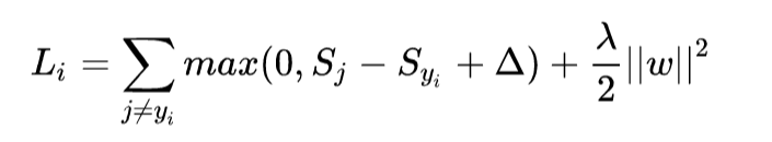
loss function 加入 regularization 项
def svm_loss_naive(W, X, y, reg):
  """
  Structured SVM loss function, naive implementation (with loops).

  Inputs have dimension D, there are C classes, and we operate on minibatches
  of N examples.

  Inputs:
  - W: A numpy array of shape (D, C) containing weights.
  - X: A numpy array of shape (N, D) containing a minibatch of data.
  - y: A numpy array of shape (N,) containing training labels; y[i] = c means
    that X[i] has label c, where 0 <= c < C.
  - reg: (float) regularization strength

  Returns a tuple of:
  - loss as single float
  - gradient with respect to weights W; an array of same shape as W
  """
  dW = np.zeros(W.shape) # initialize the gradient as zero

  # compute the loss and the gradient
  num_classes = W.shape[1]
  num_train = X.shape[0]
  loss = 0.0
  for i in range(num_train):
    scores = X[i].dot(W)
    correct_class_score = scores[y[i]]
    for j in range(num_classes):
      if j == y[i]:
        continue
      margin = scores[j] - correct_class_score + 1 # note delta = 1
      if margin > 0:
        loss += margin
        # 在loss function上分别对 W[Y[i]] 和 W[j] 求导得
        dW[:,y[i]] += -X[i,:].T
        dW[:,j] += X[i,:].T

  # Right now the loss is a sum over all training examples, but we want it
  # to be an average instead so we divide by num_train.
  loss /= num_train
  dW /= num_train

  # Add regularization to the loss.
  loss += reg * np.sum(W * W)
  dW += reg * W

  #############################################################################
  # TODO:                                                                     #
  # Compute the gradient of the loss function and store it dW.                #
  # Rather that first computing the loss and then computing the derivative,   #
  # it may be simpler to compute the derivative at the same time that the     #
  # loss is being computed. As a result you may need to modify some of the    #
  # code above to compute the gradient.                                       #
  #############################################################################


return loss, dW- 接下来,用数值梯度来验证上面所得结果
# 比较数值梯度和解析梯度
f = lambda w: svm_loss_naive(w, X_dev, y_dev, 0.0)[0]
grad_numerical = grad_check_sparse(f, W, grad)

# do the gradient check once again with regularization turned on
print('turn on reg')
loss, grad = svm_loss_naive(W, X_dev, y_dev, 5e1)
f = lambda w: svm_loss_naive(w, X_dev, y_dev, 5e1)[0]
grad_numerical = grad_check_sparse(f, W, grad)
grad_check_sparse在 gradient_check.py 中
def grad_check_sparse(f, x, analytic_grad, num_checks=10, h=1e-5):
  """
  sample a few random elements and only return numerical
  in this dimensions.
  """

  for i in range(num_checks):
    # 随机取出 W 中的一个数
    ix = tuple([randrange(m) for m in x.shape])

    # 计算数值梯度
    oldval = x[ix]
    x[ix] = oldval + h # increment by h
    fxph = f(x) # evaluate f(x + h)
    x[ix] = oldval - h # increment by h
    fxmh = f(x) # evaluate f(x - h)
    x[ix] = oldval # reset

    # 计算数值梯度和解析梯度的差值
    grad_numerical = (fxph - fxmh) / (2 * h)
    grad_analytic = analytic_grad[ix]
    rel_error = abs(grad_numerical - grad_analytic) / (abs(grad_numerical) + abs(grad_analytic))
    print('numerical: %f analytic: %f, relative error: %e' % (grad_numerical, grad_analytic, rel_error))
- 完成基于SVM的全向量化损失函数,完成解析梯度的全向量化表示
# 完成一个基于SVM的全向量化损失函数 loss
# 完成解析梯度的全向量化表示 grad
tic = time.time()
loss_naive, grad_naive = svm_loss_naive(W, X_dev, y_dev, 0.000005)
toc = time.time()
print('Naive loss: %e computed in %fs' % (loss_naive, toc - tic))

from cs231n.classifiers.linear_svm import svm_loss_vectorized
tic = time.time()
loss_vectorized, _ = svm_loss_vectorized(W, X_dev, y_dev, 0.000005)
toc = time.time()
print('Vectorized loss: %e computed in %fs' % (loss_vectorized, toc - tic))

# The losses should match but your vectorized implementation should be much faster.
print('difference: %f' % (loss_naive - loss_vectorized))

# Complete the implementation of svm_loss_vectorized, and compute the gradient
# of the loss function in a vectorized way.

# The naive implementation and the vectorized implementation should match, but
# the vectorized version should still be much faster.
tic = time.time()
_, grad_naive = svm_loss_naive(W, X_dev, y_dev, 0.000005)
toc = time.time()
print('Naive loss and gradient: computed in %fs' % (toc - tic))

tic = time.time()
_, grad_vectorized = svm_loss_vectorized(W, X_dev, y_dev, 0.000005)
toc = time.time()
print('Vectorized loss and gradient: computed in %fs' % (toc - tic))

# The loss is a single number, so it is easy to compare the values computed
# by the two implementations. The gradient on the other hand is a matrix, so
# we use the Frobenius norm to compare them.
difference = np.linalg.norm(grad_naive - grad_vectorized, ord='fro')
print('difference: %f' % difference)
svm_loss_vectorized 在 linear_svm.py中实现
def svm_loss_vectorized(W, X, y, reg):
  """
  Structured SVM loss function, vectorized implementation.

  Inputs and outputs are the same as svm_loss_naive.
  """
  loss = 0.0
  dW = np.zeros(W.shape) # initialize the gradient as zero

  #############################################################################
  # TODO:                                                                     #
  # Implement a vectorized version of the structured SVM loss, storing the    #
  # result in loss.                                                           #
  #############################################################################
  # 实现结构化SVM损失函数的向量版本
  scores = X.dot(W)                           # 得到一个 num_train * 10的矩阵
  num_classes = W.shape[1]
  num_train = X.shape[0]

  scores_correct = scores[np.arange(num_train), y]      # 用一个list小技巧直接取出所有的 scores[y[i]]
  scores_correct = np.reshape(scores_correct, (num_train, -1))

  margins = scores - scores_correct + 1
  margins = np.maximum(0, margins)
  margins[np.arange(num_train), y] = 0
  loss += np.sum(margins) / num_train
  loss += 0.5 * reg * np.sum(W * W)

  #############################################################################
  #                             END OF YOUR CODE                              #
  #############################################################################


  #############################################################################
  # TODO:                                                                     #
  # Implement a vectorized version of the gradient for the structured SVM     #
  # loss, storing the result in dW.                                           #
  #                                                                           #
  # Hint: Instead of computing the gradient from scratch, it may be easier    #
  # to reuse some of the intermediate values that you used to compute the     #
  # loss.                                                                     #
  #############################################################################
  margins[margins > 0] = 1
  row_sum = np.sum(margins, axis=1)
  margins[np.arange(num_train), y] = -row_sum
  dW += np.dot(X.T, margins) / num_train + reg * W
  #############################################################################
  #                             END OF YOUR CODE                              #
  #############################################################################

  return loss, dW
- 使用SGD,进行训练
# SGD
from cs231n.classifiers import LinearSVM
svm = LinearSVM()
tic = time.time()
loss_hist = svm.train(X_train, y_train, learning_rate=1e-7, reg=2.5e4,
                      num_iters=1500, verbose=True)
toc = time.time()
print('That took %fs' % (toc - tic))

# 画出loss曲线
plt.plot(loss_hist)
plt.xlabel('Iteration number')
plt.ylabel('Loss value')
plt.show()

# 查看正确率
y_train_pred = svm.predict(X_train)
print('training accuracy: %f' % (np.mean(y_train == y_train_pred), ))
y_val_pred = svm.predict(X_val)
print('validation accuracy: %f' % (np.mean(y_val == y_val_pred), ))
画出损失曲线

训练过程在 linear_classifier.py 中的 train函数中, 在predict函数中预测
  def train(self, X, y, learning_rate=1e-3, reg=1e-5, num_iters=100,
            batch_size=200, verbose=False):
    """
    Train this linear classifier using stochastic gradient descent.

    Inputs:
    - X: A numpy array of shape (N, D) containing training data; there are N
      training samples each of dimension D.
    - y: A numpy array of shape (N,) containing training labels; y[i] = c
      means that X[i] has label 0 <= c < C for C classes.
    - learning_rate: (float) learning rate for optimization.
    - reg: (float) regularization strength.
    - num_iters: (integer) number of steps to take when optimizing
    - batch_size: (integer) number of training examples to use at each step.
    - verbose: (boolean) If true, print progress during optimization.

    Outputs:
    A list containing the value of the loss function at each training iteration.
    """
    num_train, dim = X.shape
    num_classes = np.max(y) + 1 # assume y takes values 0...K-1 where K is number of classes
    if self.W is None:
      # lazily initialize W
      self.W = 0.001 * np.random.randn(dim, num_classes)

    # Run stochastic gradient descent to optimize W
    loss_history = []
    for it in range(num_iters):
      X_batch = None
      y_batch = None

      #########################################################################
      # TODO:                                                                 #
      # Sample batch_size elements from the training data and their           #
      # corresponding labels to use in this round of gradient descent.        #
      # Store the data in X_batch and their corresponding labels in           #
      # y_batch; after sampling X_batch should have shape (dim, batch_size)   #
      # and y_batch should have shape (batch_size,)                           #
      #                                                                       #
      # Hint: Use np.random.choice to generate indices. Sampling with         #
      # replacement is faster than sampling without replacement.              #
      #########################################################################
      batch_inx = np.random.choice(num_train, batch_size)
      X_batch = X[batch_inx,:]
      y_batch = y[batch_inx]
      #########################################################################
      #                       END OF YOUR CODE                                #
      #########################################################################

      # evaluate loss and gradient
      loss, grad = self.loss(X_batch, y_batch, reg)
      loss_history.append(loss)

      # perform parameter update
      #########################################################################
      # TODO:                                                                 #
      # Update the weights using the gradient and the learning rate.          #
      #########################################################################
      self.W = self.W - learning_rate * grad
      #########################################################################
      #                       END OF YOUR CODE                                #
      #########################################################################

      if verbose and it % 100 == 0:
        print('iteration %d / %d: loss %f' % (it, num_iters, loss))

    return loss_history

  def predict(self, X):
    """
    Use the trained weights of this linear classifier to predict labels for
    data points.

    Inputs:
    - X: A numpy array of shape (N, D) containing training data; there are N
      training samples each of dimension D.

    Returns:
    - y_pred: Predicted labels for the data in X. y_pred is a 1-dimensional
      array of length N, and each element is an integer giving the predicted
      class.
    """
    y_pred = np.zeros(X.shape[0])
    ###########################################################################
    # TODO:                                                                   #
    # Implement this method. Store the predicted labels in y_pred.            #
    ###########################################################################
    pred = np.dot(X, self.W)
    y_pred = np.argmax(pred,axis=1)
    ###########################################################################
    #                           END OF YOUR CODE                              #
    ###########################################################################
return y_pred- 接下来,调优超参 ( learning rate 和 regularization )
找出最好的 learning rate 和 regularization,构建最好的svm(W)
# 使用验证集去调超参数(lr, reg)
learning_rates = [2e-7, 1.75e-7, 1.5e-7, 1.25e-7, 1e-7, 0.75e-7]
regularization_strengths = [2e4, 2.5e4, 2.75e4, 3e4, 3.25e4, 3.5e4, 3.75e4, 4e4, 4.25e4]

results = {}
best_val = -1
best_svm = None

# 验证过程
for rate in learning_rates:
    for regular in regularization_strengths:
        svm = LinearSVM()
        svm.train(X_train, y_train, learning_rate=rate, reg=regular, num_iters=1000)  #  num_iters可以设小一点
        y_train_pred = svm.predict(X_train)
        acc_train = np.mean(y_train_pred == y_train)
        y_val_pred = svm.predict(X_val)
        acc_val = np.mean(y_val_pred == y_val)
        results[(rate, regular)] = (acc_train, acc_val)
        if best_val < acc_val:
            best_val = acc_val
            best_svm = svm

for lr, reg in sorted(results):
    train_accuracy, val_accuracy = results[(lr, reg)]
    print('lr %e reg %e train accuracy: %f val accuracy: %f' % (
        lr, reg, train_accuracy, val_accuracy))

print('best validation accuracy achieved during cross-validation: %f' % best_val)
可视化调参结果
import math
x_scatter = [math.log10(x[0]) for x in results]
y_scatter = [math.log10(x[1]) for x in results]

# plot training accuracy
marker_size = 100
colors = [results[x][0] for x in results]
plt.subplot(2, 1, 1)
plt.scatter(x_scatter, y_scatter, marker_size, c=colors)
plt.colorbar()
plt.xlabel('log learning rate\n')
plt.ylabel('log regularization strength')
plt.title('CIFAR-10 training accuracy')

# plot validation accuracy
colors = [results[x][1] for x in results] # default size of markers is 20
plt.subplot(2, 1, 2)
plt.scatter(x_scatter, y_scatter, marker_size, c=colors)
plt.colorbar()
plt.xlabel('log learning rate')
plt.ylabel('log regularization strength')
plt.title('\nCIFAR-10 validation accuracy')
plt.show()

- 使用最优的 svm 测试
# Evaluate the best svm on test set
y_test_pred = best_svm.predict(X_test)
test_accuracy = np.mean(y_test == y_test_pred)
print('linear SVM on raw pixels final test set accuracy: %f' % test_accuracy)
- 可视化最优的Weight
# 最后,取出 W 中的“标准模板”查看一下
w = best_svm.W[:-1, :]  # 丢掉 bias
w = w.reshape(32, 32, 3, 10)
w_min, w_max = np.min(w), np.max(w)
classes = ['plane', 'car', 'bird', 'cat', 'deer', 'dog', 'frog', 'horse', 'ship', 'truck']
for i in range(10):
    plt.subplot(2, 5, i + 1)

    # Rescale the weights to be between 0 and 255
    wimg = 255.0 * (w[:, :, :, i].squeeze() - w_min) / (w_max - w_min)
    plt.imshow(wimg.astype('uint8'))
    plt.axis('off')
    plt.title(classes[i])
plt.show()
可以在参数W模板中看出识别目标大致的样子