机器学习（Machine Learning）- 吴恩达（Andrew Ng） 学习笔记（七）

Regularization 正则化

The problem of overfitting 过拟合问题

什么是过拟合问题、利用正则化技术改善或者减少过拟合问题。

Example: Linear regression (housing prices) 线性回归中的过拟合

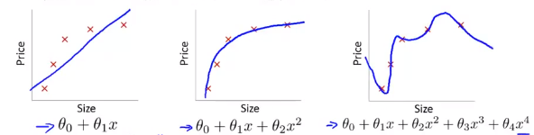
对5个训练集建立线性回归模型，分别进行如下图所示的三种分析。

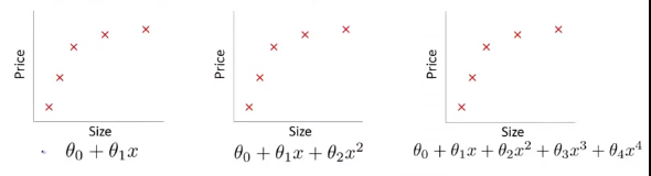
如果拟合一条直线到训练数据（图一），会出现欠拟合(underfitting)/高偏差(high bias)现象（指没有很好地拟合训练数据）。
试着拟合一个二次函数的曲线（图二），符合各项要求。称为just right。
接着拟合一个四次函数的曲线（图三），虽然曲线对训练数据做了一个很好的拟合，但是显然是不合实际的，这种情况就叫做过拟合或高方差(variance)。

Overfitting: If we have too many features, the learned hypothesis may fit the training set very well(\(\sum_{i=1}^m(h_\theta(x^{(i)}) - y^{(i)})^2 \approx 0\)), but fail to generalize to new example and fails to predict prices on new examples.

过拟合：在变量过多时训练处的方程总能很好的拟合训练数据（这时你的代价函数会非常接近于0），但是这样的曲线千方百计的拟合训练数据，以至于它无法泛化（“泛化”指一个假设模型能够应用到新样本的能力）到新的样本中。

逻辑回归中的过拟合

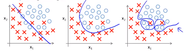
对以下训练集建立线性逻辑模型，分别进行如下图所示的三种分析。

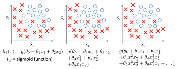
图一：欠拟合。
图二：Just Right。
图三：过拟合。

Addressing overfitting 解决过度拟合

1. Reduce number of features. 减少变量选取的数量

   —— Manually select which features to keep. 人工检查决定变量去留

   —— Model selection algorithm (later in course). 模型选择算法：自动选择采取哪些特征变量，自动舍弃不需要的变量（后续课程会讲到）

2. Regularization. 正则化

   —— Keep all the features, but reduce magnitude values of parameters \(\theta_j\).保留所有特征变量，但是减小参数\(\theta_j\)的数量级。

   —— Works well when we have a lot of features, each of which contributes a bit to predicting \(y\). 在我们拥有大量的有用特征时往往非常有效。

Cost function 通过控制代价函数实现正则化

Intuition

在我们进行拟合时，假如选择了4次函数，那我们可以通过对 \(\theta_3,\theta_4\) 加上惩罚系数影响代价函数的大小从而达到控制 \(\theta_3,\theta_4\) 大小的目的。

Suppose we penalize and make \(\theta_3,\theta_4\) really small.

\(\rightarrow\) \(min_\theta\frac{1}{2m}\sum_{i = 1}^m(h_\theta(x^{(i)}) - y^{(i)})^2 + 1000\theta_3^2 + 1000\theta_4^2\)

Regularization

Small values for parameters \(\theta_0,\theta_1,\ldots,\theta_n\)
如果我们的参数\(\theta\)值都比较小那么我们将会：
—— "Simpler" hypothesis 得到形式更简单的假设函数
—— Less prone to overfitting 不易发生过拟合的情况（因为\(\theta\)值越小，对应曲线越光滑）

Housing:
—— Features: \(x_1, x_2. \ldots, x_{100}\)
—— parameters: \(\theta_0,\theta_1,\theta_2,\ldots,\theta_{100}\)

In regularized linear regression, we choose \(\theta\) to minimize
\(J(\theta) = \frac{1}{2m}\left[\sum_{i=1}^m(h_\theta(x^{(i)})-y^{(i)})^2+\lambda\sum_{i=1}^n\theta_j^2\right]\).
最后一项称为正则化项，\(\lambda\)称为正则化参数。

What if \(\lambda\) is set to an extremely large value (perhaps for too large for our problem, say \(\lambda = 10^{10}\))?
如果\(\lambda\)设置的太大的话，\(\theta_1, \ldots, \theta_n\)将会接近于0，此时的函数图像接近一条水平直线，对于数据来说就是欠拟合了。

Regularized linear regression 应用正则化到线性回归中

梯度下降法

在原来的算法基础上略微改动：把\(\theta_0\)的更新单独取出来并加入正则化项，如下：

Repeat{
\(\theta_0 := \theta_0 - \alpha\frac{1}{m}\sum_{i=1}^m(h_\theta(x^{(i)})-y^{(i)})x_0^{(i)}\)
\(\theta_j := \theta_j - \alpha\frac{1}{m}\left[ \sum_{i=1}^m(h_\theta(x^{(i)})-y^{(i)})x_j^{(i)}+\lambda\theta_j\right]\) (j = 1,2,3,...,n)
}

\(\theta_0\)单独取出来的原因是：对于正则化的线性回归，我们的惩罚参数不包含\(\theta_0\)。

上式中的第二项也可以写为：\(\theta_j := \theta_j (1- \alpha\frac{\lambda}{m}) - \alpha\frac{1}{m}\sum_{i=1}^m(h_\theta(x^{(i)})-y^{(i)})x_j^{(i)}\)

Normal equation 正规方程

\(X= \left[ \begin{matrix} (x^{(1)})^T \\ \vdots \\ (x^{(m)})^T \end{matrix} \right]\) \(y = \left[ \begin{matrix} (y^{(1)})^T \\ \vdots \\ (x^{(m)})^T \end{matrix} \right]\) \(\rightarrow\) \(min_\theta J(\theta)\)

\(\rightarrow\) \(\theta = (X^TX + \lambda diag(0,1,1,\ldots,1)_{(n+1)})^{-1}X^Ty\)

Non-invertibility(optional/advanced) 当矩阵不可逆时（选学）

Suppose \(m \leq n\), \(\theta = (X^TX)^{-1}X^Ty\)
If \(\lambda > 0\), \(\theta = X^TX + \lambda diag(0,1,1,\ldots,1)_{(n+1)}^{-1}X^Ty\)

Regularized logistic regression 应用正则化到逻辑回归中

如何改进梯度下降算法和高级优化算法使其能够应用于正则化的逻辑回归。

Cost function:

\(J(\theta) = -\left[ \frac{1}{m}\sum_{i=1}^my^{(i)}log h_\theta(x^{(i)}) + (1-y^{(i)})log(1-h_\theta(x^{(i)})) \right] + \frac{\lambda}{2m}\sum_{j=1}^n\theta_j^2|(\theta_1,\theta_2,\ldots,\theta_n)\)

具体实现如下，其中\(h_\theta(x) = \frac{1}{1+e^{-\theta^Tx}}\).

Repeat{
\(\theta_0 := \theta_0 - \alpha\frac{1}{m}\sum_{i=1}^m(h_\theta(x^{(i)})-y^{(i)})x_0^{(i)}\)
\(\theta_j := \theta_j - \alpha\frac{1}{m}\left[ \sum_{i=1}^m(h_\theta(x^{(i)})-y^{(i)})x_j^{(i)}+\lambda\theta_j\right]\) (j = 1,2,3,...,n)
}

Advanced optimization 高级优化算法

自定义的函数（伪代码）：

function [jVal, gradient] = costFunction(theta)
jval = [code to compute J(\(\theta\))]
gradient(1) = [code to compute \(\frac{\partial}{\partial\theta_0}J(\theta)\)]
gradient(2) = [code to compute \(\frac{\partial}{\partial\theta_1}J(\theta)\)]
gradient(3) = [code to compute \(\frac{\partial}{\partial\theta_2}J(\theta)\)]
\(\vdots\)
gradient(n+1) = [code to compute \(\frac{\partial}{\partial\theta_n}J(\theta)\)]

其中：

1. code to compute J(\(\theta\))：\(J(\theta) = -\left[ \frac{1}{m}\sum_{i=1}^my^{(i)}log h_\theta(x^{(i)}) + (1-y^{(i)})log(1-h_\theta(x^{(i)})) \right] + \frac{\lambda}{2m}\sum_{j=1}^n\theta_j^2\)
2. code to compute \(\frac{\partial}{\partial\theta_0} J(\theta)\)：\(\frac{1}{m}\sum_{i=1}^m(h_\theta(x^{(i)}) - y^{(i)})x_0^{(i)}\)
3. code to compute \(\frac{\partial}{\partial\theta_1} J(\theta)\)：\(\frac{1}{m}\sum_{i=1}^m(h_\theta(x^{(i)}) - y^{(i)})x_1^{(i)} + \frac{\lambda}{m}\theta_1\)
4. code to compute \(\frac{\partial}{\partial\theta_2} J(\theta)\)：\(\frac{1}{m}\sum_{i=1}^m(h_\theta(x^{(i)}) - y^{(i)})x_2^{(i)} + \frac{\lambda}{m}\theta_2\)

剩下要做的是将自定义函数带入到fminunc函数中。