机器学习（Machine Learning）- 吴恩达（Andrew Ng） 学习笔记（二）

Liner regression with one variable

Model Representation 模型表示

Supervised Learning 监督学习

Given the "right answer" for each example in the data. 对每个数据来说，我们给出了”正确答案“。

Regression Problem 回归问题

Predict real-valued output. 我们根据之前的数据预测出一个准确的输出值。

Training set 训练集

Notation： 常见符号表示

1. m = Number of training examples 训练样本
2. x = "input" variable / feature 输入变量 / 特征值
3. y = "output" variable / "target" variable 输出变量 / 目标变量
4. (x, y) = one training example 一个训练样本
5. (\(x^i, y^i\)) = the \(i_{th}\) training example 第i个训练样本

hypothesis 假设（是一个函数）

1. Training set -> Learning Algorithm -> h 将数据集“喂”给学习算法，学习算法输出一个函数。

2. x -> h -> y a map from \(x's\) to \(y's\). 是一个从x到y的映射函数。

3. How do we represent h?

   \(h_{\theta}(x) = \theta_0 + \theta_1 \times x\).

Summery

数据集和函数的作用：预测一个关于x的线性函数y

Cost function 代价函数

如何把最有可能的直线与我们的数据相拟合

Idea

Choose \(\theta_0, \theta_1\) so that \(h_{\theta}(x)\) is close to \(y\) for our training examples (\(x, y\)).

Squared error function

\(J(\theta_0, \theta_1) = \frac{1}{2m} \sum_{i=1}^m(h_{\theta}(x^i) - y^i)^2\)

目标：找到\(\theta_0,\theta_1\) 使得 \(J(\theta_0, \theta_1)\)最小。其中\(J(\theta_0, \theta_1)\)称为代价函数

Cost function intuition

Review

1. Hypothesis: \(h_{\theta}(x) = \theta_0 + \theta_1 \times x\)
2. Parameters: \(\theta_0, \theta_1\)
3. Cost Function: \(J(\theta_0, \theta_1) = \frac{1}{2m} \sum_{i=1}^m(h_{\theta}(x^i) - y^i)^2\)
4. Goal: find \(\theta_0,\theta_1\) to minimize \(J(\theta_0, \theta_1)\)

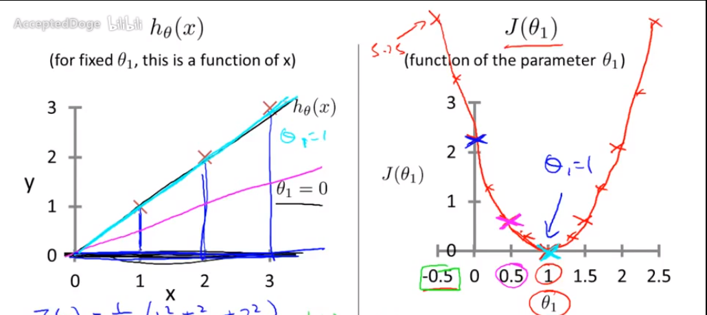
Simplified

\(\theta_0 = 0 \rightarrow h_{\theta}(x) = \theta_1x\)

\(J(\theta_1) = \frac{1}{2m} \sum_{i=1}^m(h_{\theta}(x^i) - y^i)^2\)

Goal: find \(\theta_1\) to minimize \(J(\theta_1)\)

例子：样本点包含(1, 1)、(2, 2)、(3, 3)的假设函数和代价函数的关系图

Gradient descent 梯度下降

Background

Have some function \(J(\theta_0, \theta_1, \theta_2, \ldots, \theta_n)\)

Want find \(\theta_0, \theta_1, \theta_2, \ldots, \theta_n\) to minimize \(J(\theta_0, \theta_1, \theta_2, \ldots, \theta_n)\)

Simplify -> \(\theta_1, \theta_2\)

Outline

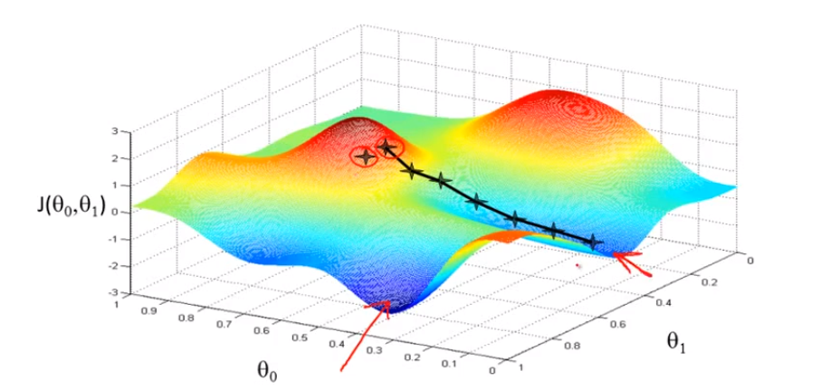
1. start with some \(\theta_0, \theta_1\) (\(\theta_0 = 0, \theta_1 = 0\)). 初始化
2. Keep changing \(\theta_0, \theta_1\) to reduce \(J(\theta_0, \theta_1)\) until we hopefully end up at a minimum. 不断寻找最优解，直到找到局部最优解（从不同点/方向出发得到的最终结果可能会不同）。

Gradient descent algorithm

1. repeat until convergence {

   ​ \(\theta_j := \theta_j - \alpha\frac{\partial}{\partial\theta_j}J(\theta_0, \theta_1)\) (for \(j= 0\) and \(j = 1\))

   }

   变量含义：\(\alpha\): learning rate 学习速率（控制我们以多大的幅度更新这个参数\(\theta_j\) ）

2. Correct: Simultaneous update 正确实现同时更新的方法

   \(temp0 := \theta_0 - \alpha\frac{\partial}{\partial\theta_j}J(\theta_0, \theta_1)\)

   \(temp1 := \theta_1 - \alpha\frac{\partial}{\partial\theta_j}J(\theta_0, \theta_1)\)

   \(\theta_0 := temp0\)

   \(\theta_1 := temp1\)

3. Incorrect: 没有实现同步更新

   \(temp0 := \theta_0 - \alpha\frac{\partial}{\partial\theta_j}J(\theta_0, \theta_1)\)

   \(\theta_0 := temp0\)

   \(temp1 := \theta_1 - \alpha\frac{\partial}{\partial\theta_j}J(\theta_0, \theta_1)\)

   \(\theta_1 := temp1\)

Gradient descent intuition

导数项的意义

1. 当\(\alpha\frac{\partial}{\partial\theta_j}J(\theta_0, \theta_1) > 0\) （即函数处于递增状态）时，\(\because \alpha > 0\)，\(\therefore \theta_1 := \theta_1 - \alpha\frac{\partial}{\partial\theta_j}J(\theta_0, \theta_1) < 0\)，即向最低点处移动。
2. 当\(\alpha\frac{\partial}{\partial\theta_j}J(\theta_0, \theta_1) < 0\) （即函数处于递减状态）时，\(\because \alpha > 0\)，\(\therefore \theta_1 := \theta_1 - \alpha\frac{\partial}{\partial\theta_j}J(\theta_0, \theta_1) > 0\)，即向最低点处移动。

学习速率\(\alpha\)

1. If \(\alpha\) is too small, gradient descent can be slow. \(\alpha\)太小，会使梯度下降的太慢。
2. If \(\alpha\) is too large, gradient descent can overshoot the minimum. It may fail to converge, or even diverge. \(\alpha\)太大，梯度下降法可能会越过最低点，甚至可能无法收敛。

思考

1. 假设你将\(\theta_1\)初始化在局部最低点，而这条线的斜率将等于0，因此导数项等于0，梯度下降更新的过程中就会有\(\theta_1 = \theta_1\)。

2. Gradient descent can converge to a local minimum, even with the learning rate \(\alpha\) fixed. 即使学习速率\(\alpha\)固定不变，梯度下降也可以达到局部最小值。

   As we approach a local minimum, gradient descent will automatically take smaller steps. So, no need to decrease \(\alpha\) over time. 在我们接近局部最小值时，梯度下降将会自动更换为更小的步子，因此我们没必要随着时间的推移而更改\(\alpha\)的值。（因为斜率在变）

Gradient descent for linear regression 梯度下降在线性回归中的应用

化简公式

$\frac{\partial}{\partial\theta_j}J(\theta_0, \theta_1) = \frac{\partial}{\partial\theta_j} \frac{1}{2m} \sum_{i = 1}^m(h_\theta(x^i) - y^i)^2 = \frac{\partial}{\partial\theta_j} \frac{1}{2m} \sum_{i = 0}^m(\theta_0 + \theta_1x^i - y^i)^2 $

分别对\(\theta_0,\theta_1\)求偏导

1. \(j = 0\) : $ \frac{\partial}{\partial\theta_0}J(\theta_0, \theta_1) = \frac{1}{m} \sum_{i=1}^m(h_{\theta}(x^i) - y^i) $
2. \(j = 1\) : $ \frac{\partial}{\partial\theta_1}J(\theta_0, \theta_1) = \frac{1}{m} \sum_{i=1}^m(h_{\theta}(x^i) - y^i) \times x^i $

Gradient descent algorithm 将上面结果放回梯度下降法中

repeat until convergence {

​ $\theta_0 := \theta_0 - \alpha \frac{1}{m} \sum_{i=1}^m(h_{\theta}(x^i) - y^i) $

​ $\theta_1 := \theta_1 - \alpha \frac{1}{m} \sum_{i=1}^m(h_{\theta}(x^i) - y^i) \times x^i $

}

"Batch" Gradient Descent 批梯度下降法

"Batch": Each step of gradient descent uses all the training examples. 每迭代一步，都要用到训练集的所有数据。