原文链接：http://tecdat.cn/?p=9484

介绍

下面以物种多样性为例子展示了如何在R语言中进行相关分析和线性回归分析。

怎么做测试

相关和线性回归示例


Data = read.table(textConnection(Input),header=TRUE)

数据简单图

plot(Species ~ Latitude, 
     data=Data, 
     pch=16,
     xlab = "Latitude", 
     ylab = "Species")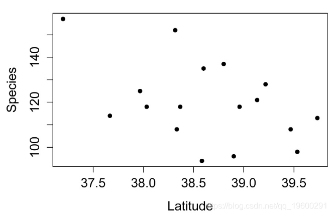

相关性

可以使用 cor.test函数。它可以执行Pearson，Kendall和Spearman相关。

皮尔逊相关

皮尔逊相关是最常见的相关形式。假设数据是线性相关的，并且残差呈正态分布。

cor.test( ~ Species + Latitude, 
         data=Data,
         method = "pearson",
         conf.level = 0.95)



Pearson's product-moment correlation



t = -2.0225, df = 15, p-value = 0.06134



       cor

-0.4628844

肯德尔相关

肯德尔秩相关是一种非参数检验，它不假设数据的分布或数据是线性相关的。它对数据进行排名以确定相关程度。

cor.test( ~ Species + Latitude, 
         data=Data,
         method = "kendall",
         continuity = FALSE,
         conf.level = 0.95)

 

Kendall's rank correlation tau

 

z = -1.3234, p-value = 0.1857

 

       tau

-0.2388326

斯皮尔曼相关

Spearman等级相关性是一种非参数检验，它不假设数据的分布或数据是线性相关的。它对数据进行排序以确定相关程度，并且适合于顺序测量。

线性回归

线性回归可以使用 lm函数执行。可以使用lmrob函数执行稳健回归。



summary(model)                    # shows parameter estimates,
                                  # p-value for model, r-square

 

            Estimate Std. Error t value Pr(>|t|) 

(Intercept)  585.145    230.024   2.544   0.0225 *

Latitude     -12.039      5.953  -2.022   0.0613 .

 

Multiple R-squared:  0.2143,  Adjusted R-squared:  0.1619

F-statistic:  4.09 on 1 and 15 DF,  p-value: 0.06134

 

 



Response: Species

          Sum Sq Df F value  Pr(>F) 

Latitude  1096.6  1  4.0903 0.06134 .

Residuals 4021.4 15

绘制线性回归


plot(Species ~ Latitude,
     data = Data,
     pch=16,
     xlab = "Latitude", 
     ylab = "Species")

abline(int, slope,
       lty=1, lwd=2, col="blue")     #  style and color of line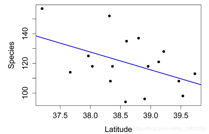

检查模型的假设

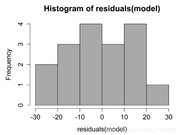
线性模型中残差的直方图。这些残差的分布应近似正态。

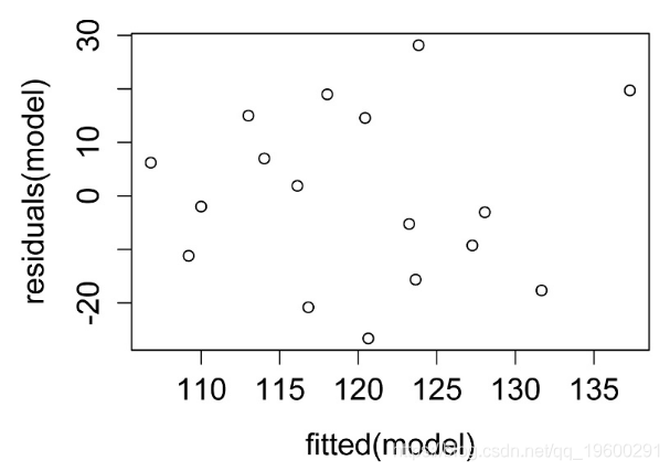
残差与预测值的关系图。残差应无偏且均等。

稳健回归

该线性回归对响应变量中的异常值不敏感。



summary(model)                    # shows parameter estimates, r-square

 

            Estimate Std. Error t value Pr(>|t|) 

(Intercept)  568.830    230.203   2.471   0.0259 *

Latitude     -11.619      5.912  -1.966   0.0681 .

 

Multiple R-squared:  0.1846,  Adjusted R-squared:  0.1302

 

 
                   
anova(model, model.null)         # shows p-value for model

 

  pseudoDf Test.Stat Df Pr(>chisq) 

1       15                         

2       16    3.8634  1    0.04935 *

绘制模型

线性回归示例



summary(model)                    # shows parameter estimates, 
                                  # p-value for model, r-square

 

Coefficients:

            Estimate Std. Error t value Pr(>|t|)  

(Intercept)  12.6890     4.2009   3.021   0.0056 **

Weight        1.6017     0.6176   2.593   0.0154 *

 

Multiple R-squared:  0.2055,  Adjusted R-squared:  0.175

F-statistic: 6.726 on 1 and 26 DF,  p-value: 0.0154

 

###  Neither the r-squared nor the p-value agrees with what is reported

###    in the Handbook.

 

 

library(car)

Anova(model, type="II")           # shows p-value for effects in model

 

          Sum Sq Df F value Pr(>F) 

Weight     93.89  1  6.7258 0.0154 *

Residuals 362.96 26  

 

#     #     #

功率分析

功率分析的相关性

### --------------------------------------------------------------
### Power analysis, correlation
### --------------------------------------------------------------

pwr.r.test()

 

     approximate correlation power calculation (arctangh transformation)

 

              n = 28.87376