原文链接:http://tecdat.cn/?p=8531
- 执行多项式回归使用
age预测wage。使用交叉验证为多项式选择最佳次数。选择了什么程度,这与使用进行假设检验的结果相比如何ANOVA?对所得多项式拟合数据进行绘图。
加载工资数据集。保留所有交叉验证错误的数组。我们正在执行K=10 K倍交叉验证。
rm(list = ls())
set.seed(1)
library(ISLR)
library(boot)

# container of test errors
cv.MSE <- NA

# loop over powers of age
for (i in 1:15) {
  glm.fit <-  glm(wage ~ poly(age, i), data = Wage)
  # we use cv.glm's cross-validation and keep the vanilla cv test error
  cv.MSE[i] <-  cv.glm(Wage, glm.fit, K = 10)$delta[1]
}
# inspect results object
cv.MSE
## [1] 1675.837 1601.012 1598.801 1594.217 1594.625 1594.888 1595.500
## [8] 1595.436 1596.335 1595.835 1595.970 1597.971 1598.713 1599.253
## [15] 1595.332我们通过绘制type = "b"点与线之间的关系图来说明结果。
# illustrate results with a line plot connecting the cv.error dots
plot( x = 1:15, y = cv.MSE, xlab = "power of age", ylab = "CV error",
      type = "b", pch = 19, lwd = 2, bty = "n",
      ylim = c( min(cv.MSE) - sd(cv.MSE), max(cv.MSE) + sd(cv.MSE) ) )

# horizontal line for 1se to less complexity
abline(h = min(cv.MSE) + sd(cv.MSE) , lty = "dotted")

# where is the minimum
points( x = which.min(cv.MSE), y = min(cv.MSE), col = "red", pch = "X", cex = 1.5 )![]()
我们再次以较高的年龄权重对模型进行拟合以进行方差分析。
## Analysis of Deviance Table
##
## Model  1: wage ~ poly(age, a)
## Model  2: wage ~ poly(age, a)
## Model  3: wage ~ poly(age, a)
## Model  4: wage ~ poly(age, a)
## Model  5: wage ~ poly(age, a)
## Model  6: wage ~ poly(age, a)
## Model  7: wage ~ poly(age, a)
## Model  8: wage ~ poly(age, a)
## Model  9: wage ~ poly(age, a)
## Model 10: wage ~ poly(age, a)
## Model 11: wage ~ poly(age, a)
## Model 12: wage ~ poly(age, a)
## Model 13: wage ~ poly(age, a)
## Model 14: wage ~ poly(age, a)
## Model 15: wage ~ poly(age, a)
##    Resid. Df Resid. Dev Df Deviance        F    Pr(>F)
## 1       2998    5022216
## 2       2997    4793430  1   228786 143.5637 < 2.2e-16 ***
## 3       2996    4777674  1    15756   9.8867  0.001681 **
## 4       2995    4771604  1     6070   3.8090  0.051070 .
## 5       2994    4770322  1     1283   0.8048  0.369731
## 6       2993    4766389  1     3932   2.4675  0.116329
## 7       2992    4763834  1     2555   1.6034  0.205515
## 8       2991    4763707  1      127   0.0795  0.778016
## 9       2990    4756703  1     7004   4.3952  0.036124 *
## 10      2989    4756701  1        3   0.0017  0.967552
## 11      2988    4756597  1      103   0.0648  0.799144
## 12      2987    4756591  1        7   0.0043  0.947923
## 13      2986    4756401  1      190   0.1189  0.730224
## 14      2985    4756158  1      243   0.1522  0.696488
## 15      2984    4755364  1      795   0.4986  0.480151
## ---
## Signif. codes:  0 '***' 0.001 '**' 0.01 '*' 0.05 '.' 0.1 ' ' 1
根据F检验,我们应该选择年龄提高到3的幂的模型,而通过交叉验证 。
现在,我们绘制多项式拟合的结果。
plot(wage ~ age, data = Wage, col = "darkgrey",  bty = "n")
...![]()
- 拟合阶跃函数以
wage使用进行预测age。绘制获得的拟合图。
cv.error <-  NA
...

# highlight minimum
points( x = which.min(cv.error), y = min(cv.error, na.rm = TRUE), col = "red", pch = "X", cex = 1.5 )![]()
k=8 k=81sd1sdk=4k=4

![]() 44
44

lm.fit <-  glm(wage ~ cut(age, 4), data = Wage)
...
matlines(age.grid, cbind( lm.pred$fit + 2* lm.pred$se.fit,
                          lm.pred$fit - 2* lm.pred$se.fit),
         col = "red", lty ="dashed")
Q2
该Wage数据集包含了一些其他的功能,我们还没有覆盖,如婚姻状况(maritl),作业类(jobclass),等等。探索其中一些其他预测变量与的关系wage,并使用非线性拟合技术将灵活的模型拟合到数据中。
...
summary(Wage[, c("maritl", "jobclass")] )
## maritl jobclass
## 1. Never Married: 648 1. Industrial :1544
## 2. Married :2074 2. Information:1456
## 3. Widowed : 19
## 4. Divorced : 204
## 5. Separated : 55# boxplots of relationships
par(mfrow=c(1,2))
plot(Wage$maritl, Wage$wage, frame.plot = "FALSE")
plot(Wage$jobclass, Wage$wage, frame.plot = "FALSE")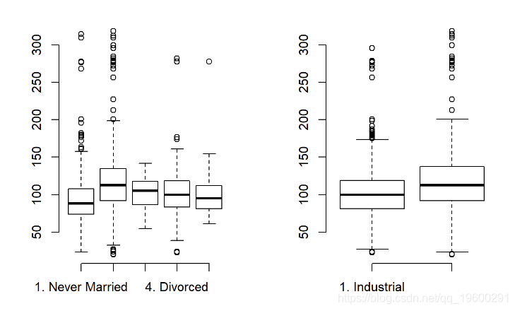
![]()
看来一对已婚夫妇平均比其他群体挣更多的钱。看来,信息性工作的工资平均高于工业性工作。
多项式和阶跃函数
m1 <-  lm(wage ~ maritl, data = Wage)
deviance(m1) # fit (RSS in linear; -2*logLik)
## [1] 4858941m2 <- lm(wage ~ jobclass, data = Wage)
deviance(m2)## [1] 4998547m3 <- lm(wage ~ maritl + jobclass, data = Wage)
deviance(m3)## [1] 4654752正如预期的那样,使用最复杂的模型可以使样本内数据拟合最小化。
我们不能使样条曲线适合分类变量。
我们不能将样条曲线拟合到因子,但可以使用一个样条曲线拟合一个连续变量并添加其他预测变量的模型。
library(gam)
m4 <-  gam(...)
deviance(m4)
## [1] 4476501anova(m1, m2, m3, m4)
## Analysis of Variance Table
##
## Model 1: wage ~ maritl
## Model 2: wage ~ jobclass
## Model 3: wage ~ maritl + jobclass
## Model 4: wage ~ maritl + jobclass + s(age, 4)
##   Res.Df     RSS      Df Sum of Sq      F    Pr(>F)
## 1   2995 4858941
## 2   2998 4998547 -3.0000   -139606 31.082 < 2.2e-16 ***
## 3   2994 4654752  4.0000    343795 57.408 < 2.2e-16 ***
## 4   2990 4476501  4.0002    178252 29.764 < 2.2e-16 ***
## ---
## Signif. codes: 0 '***' 0.001 '**' 0.01 '*' 0.05 '.' 0.1 ' ' 1F检验表明,我们从模型四送一统计显著改善计有年龄花,wage,maritl,和jobclass。
Boston数据回归
变量dis(距离五个波士顿就业中心的加权平均), nox (在每10百万份的氮氧化物浓度) 。我们将其dis视为预测因素和nox作为响应变量。
rm(list = ls())
set.seed(1)
library(MASS)
attach(Boston)
## The following objects are masked from Boston (pos = 14):
##
## age, black, chas, crim, dis, indus, lstat, medv, nox, ptratio,
## rad, rm, tax, zn- 使用
poly()函数拟合三次多项式回归来预测nox使用dis。报告回归输出,并绘制结果数据和多项式拟合。
m1 <-  lm(nox ~ poly(dis, 3))
summary(m1)
##
## Call:
## lm(formula = nox ~ poly(dis, 3))
##
## Residuals:
## Min 1Q Median 3Q Max
## -0.121130 -0.040619 -0.009738 0.023385 0.194904
##
## Coefficients:
## Estimate Std. Error t value Pr(>|t|)
## (Intercept) 0.554695 0.002759 201.021 < 2e-16 ***
## poly(dis, 3)1 -2.003096 0.062071 -32.271 < 2e-16 ***
## poly(dis, 3)2 0.856330 0.062071 13.796 < 2e-16 ***
## poly(dis, 3)3 -0.318049 0.062071 -5.124 4.27e-07 ***
## ---
## Signif. codes: 0 '***' 0.001 '**' 0.01 '*' 0.05 '.' 0.1 ' ' 1
##
## Residual standard error: 0.06207 on 502 degrees of freedom
## Multiple R-squared: 0.7148, Adjusted R-squared: 0.7131
## F-statistic: 419.3 on 3 and 502 DF, p-value: < 2.2e-16dislim <- range(dis)
...
lines(x = dis.grid, y = lm.pred$fit, col = "red", lwd = 2)
matlines(x = dis.grid, y = cbind(lm.pred$fit + 2* lm.pred$se.fit,
lm.pred$fit - 2* lm.pred$se.fit)
, col = "red", lwd = 1.5, lty = "dashed")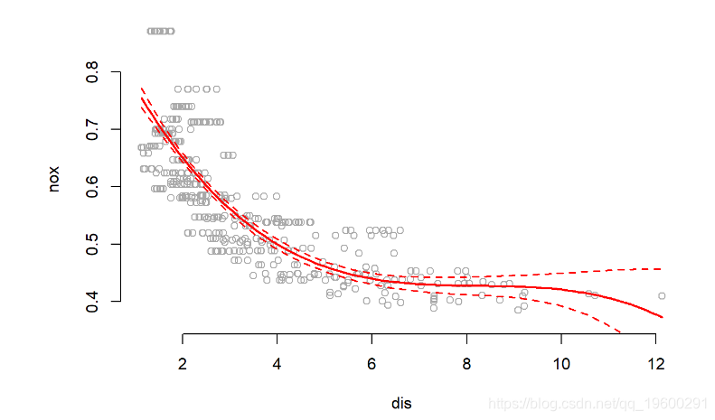
![]()
摘要显示,在nox使用进行预测时,所有多项式项都是有效的dis。该图显示了一条平滑的曲线,很好地拟合了数据。
- 绘制多项式适合不同多项式度的范围(例如,从1到10),并报告相关的残差平方和。
我们绘制1到10度的多项式并保存RSS。
# container
train.rss <-  NA
...
# show model fit in training set
train.rss
## [1] 2.768563 2.035262 1.934107 1.932981 1.915290 1.878257 1.849484
## [8] 1.835630 1.833331 1.832171正如预期的那样,RSS随多项式次数单调递减。
- 执行交叉验证或其他方法来选择多项式的最佳次数,并解释您的结果。
我们执行LLOCV并手工编码:
# container
cv.error <- matrix(NA, nrow = nrow(Boston), ncol = 10)

...
names(result) <- paste( "^", 1:10, sep= "" )
result
## ^1 ^2 ^3 ^4 ^5 ^6
## 0.005471468 0.004022257 0.003822345 0.003820121 0.003785158 0.003711971
## ^7 ^8 ^9 ^10
## 0.003655106 0.003627727 0.003623183 0.003620892plot(result ~ seq(1,10), type = "b", pch = 19, bty = "n", xlab = "powers of dist to empl. center",
ylab = "cv error")
abline(h = min(cv.error) + sd(cv.error), col = "red", lty = "dashed")![]()
基于交叉验证,我们将选择dis平方。
- 使用
bs()函数拟合回归样条曲线以nox使用进行预测dis。使用四个自由度报告适合度的输出。
[3,6,9][3,6,9]bs()dfknots
library(splines)
m4 <-  lm(nox ~ bs(dis, knots = c(3, 6, 9)))
summary(m4)
##
## Call:
## lm(formula = nox ~ bs(dis, knots = c(3, 6, 9)))
##
## Residuals:
## Min 1Q Median 3Q Max
## -0.132134 -0.039466 -0.009042 0.025344 0.187258
##
## Coefficients:
## Estimate Std. Error t value Pr(>|t|)
## (Intercept) 0.709144 0.016099 44.049 < 2e-16 ***
## bs(dis, knots = c(3, 6, 9))1 0.006631 0.025467 0.260 0.795
## bs(dis, knots = c(3, 6, 9))2 -0.258296 0.017759 -14.544 < 2e-16 ***
## bs(dis, knots = c(3, 6, 9))3 -0.233326 0.027248 -8.563 < 2e-16 ***
## bs(dis, knots = c(3, 6, 9))4 -0.336530 0.032140 -10.471 < 2e-16 ***
## bs(dis, knots = c(3, 6, 9))5 -0.269575 0.058799 -4.585 5.75e-06 ***
## bs(dis, knots = c(3, 6, 9))6 -0.303386 0.062631 -4.844 1.70e-06 ***
## ---
## Signif. codes: 0 '***' 0.001 '**' 0.01 '*' 0.05 '.' 0.1 ' ' 1
##
## Residual standard error: 0.0612 on 499 degrees of freedom
## Multiple R-squared: 0.7244, Adjusted R-squared: 0.7211
## F-statistic: 218.6 on 6 and 499 DF, p-value: < 2.2e-16# plot results
...
# all lines at once
matlines( dis.grid,
...
col = "black", lwd = 2, lty = c("solid", "dashed", "dashed"))![]()
dis>9dis>9
- 现在针对一定范围的自由度拟合样条回归,并绘制结果拟合并报告结果RSS。描述获得的结果。
我们使用3到16之间的dfs拟合回归样条曲线。
box <-  NA

for (i in 3:16) {
...
}

box[-c(1, 2)]
## [1] 1.934107 1.922775 1.840173 1.833966 1.829884 1.816995 1.825653
## [8] 1.792535 1.796992 1.788999 1.782350 1.781838 1.782798 1.783546df=14df=14
ISLR包中的College数据集。
- 将数据分为训练集和测试集。使用学费作为响应,使用其他变量作为预测变量,对训练集执行前向逐步选择,以便确定仅使用预测变量子集的令人满意的模型。
rm(list = ls())
set.seed(1)
library(leaps)
attach(College)
## The following objects are masked from College (pos = 14):
##
## Accept, Apps, Books, Enroll, Expend, F.Undergrad, Grad.Rate,
## Outstate, P.Undergrad, perc.alumni, Personal, PhD, Private,
## Room.Board, S.F.Ratio, Terminal, Top10perc, Top25perc# train/test split row index numbers
train <- sample( length(Outstate), length(Outstate)/2)
test <- -train
...
abline(h=max.adjr2 - std.adjr2, col="red", lty=2)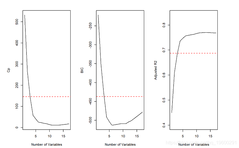
![]()
所有cp,BIC和adjr2得分均显示大小6是该子集的最小大小。但是,根据1个标准误差规则,我们将选择具有4个预测变量的模型。
...
coefi <-  coef(m5, id = 4)
names(coefi)
## [1] "(Intercept)" "PrivateYes" "Room.Board" "perc.alumni" "Expend"- 将GAM拟合到训练数据上,使用州外学费作为响应,并使用在上一步中选择的功能作为预测变量。绘制结果,并解释您的发现。
library(gam)
...
plot(gam.fit, se=TRUE, col="blue")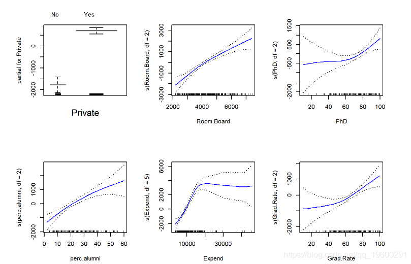
![]()
- 评估在测试集上获得的模型,并解释获得的结果。
gam.pred <-  predict(gam.fit, College.test)
gam.err <-  mean((College.test$Outstate - gam.pred)^2)
gam.err
## [1] 3745460gam.tss <- mean((College.test$Outstate - mean(College.test$Outstate))^2)
test.rss <- 1 - gam.err / gam.tss
test.rss## [1] 0.76969160.770.770.740.74
- 对于哪些变量(如果有),是否存在与响应呈非线性关系的证据?
summary(gam.fit)
##
## Call: gam(formula = Outstate ~ Private + s(Room.Board, df = 2) + s(PhD,
##     df = 2) + s(perc.alumni, df = 2) + s(Expend, df = 5) + s(Grad.Rate,
##     df = 2), data = College.train)
## Deviance Residuals:
##      Min       1Q   Median       3Q      Max
## -4977.74 -1184.52    58.33  1220.04  7688.30
##
## (Dispersion Parameter for gaussian family taken to be 3300711)
##
##     Null Deviance: 6221998532 on 387 degrees of freedom
## Residual Deviance: 1231165118 on 373 degrees of freedom
## AIC: 6941.542
##
## Number of Local Scoring Iterations: 2
##
## Anova for Parametric Effects
##                         Df     Sum Sq    Mean Sq F value    Pr(>F)
## Private                  1 1779433688 1779433688 539.106 < 2.2e-16 ***
## s(Room.Board, df = 2)    1 1221825562 1221825562 370.171 < 2.2e-16 ***
## s(PhD, df = 2)           1  382472137  382472137 115.876 < 2.2e-16 ***
## s(perc.alumni, df = 2)   1  328493313  328493313  99.522 < 2.2e-16 ***
## s(Expend, df = 5)        1  416585875  416585875 126.211 < 2.2e-16 ***
## s(Grad.Rate, df = 2)     1   55284580   55284580  16.749 5.232e-05 ***
## Residuals              373 1231165118    3300711
## ---
## Signif. codes:  0 '***' 0.001 '**' 0.01 '*' 0.05 '.' 0.1 ' ' 1
##
## Anova for Nonparametric Effects
##                        Npar Df  Npar F     Pr(F)
## (Intercept)
## Private
## s(Room.Board, df = 2)        1  3.5562   0.06010 .
## s(PhD, df = 2)               1  4.3421   0.03786 *
## s(perc.alumni, df = 2)       1  1.9158   0.16715
## s(Expend, df = 5)            4 16.8636 1.016e-12 ***
## s(Grad.Rate, df = 2)         1  3.7208   0.05450 .
## ---
## Signif. codes:  0 '***' 0.001 '**' 0.01 '*' 0.05 '.' 0.1 ' ' 1
非参数Anova检验显示了响应与支出之间存在非线性关系的有力证据,以及响应与Grad.Rate或PhD之间具有中等强度的非线性关系(使用p值为0.05)。
如果您有任何疑问,请在下面发表评论。
大数据部落 -中国专业的第三方数据服务提供商,提供定制化的一站式数据挖掘和统计分析咨询服务
统计分析和数据挖掘咨询服务:y0.cn/teradat(咨询服务请联系官网客服)
![]()
QQ:3025393450
![]() QQ交流群:186388004
QQ交流群:186388004 
【服务场景】
科研项目; 公司项目外包;线上线下一对一培训;数据爬虫采集;学术研究;报告撰写;市场调查。
【大数据部落】提供定制化的一站式数据挖掘和统计分析咨询


欢迎选修我们的R语言数据分析挖掘必知必会课程!

大数据部落 -中国专业的第三方数据服务提供商,提供定制化的一站式数据挖掘和统计分析咨询服务
统计分析和数据挖掘咨询服务:y0.cn/teradat(咨询服务请联系官网客服)
![]()
QQ:3025393450
![]() QQ交流群:186388004
QQ交流群:186388004
【服务场景】
科研项目; 公司项目外包;线上线下一对一培训;数据爬虫采集;学术研究;报告撰写;市场调查。
【大数据部落】提供定制化的一站式数据挖掘和统计分析咨询
欢迎选修我们的R语言数据分析挖掘必知必会课程!