经典的卷积神经网络结构总结

概览

本文将介绍几种经典的卷积神经网络模型，包括 LeNet-5，AlexNet，ResNet，VGGNet。
一般架构如下

• 定义超参数
  epoch，batch_size
• 定义函数进行网络架构
  初始化权重参数
• 构建计算图
  节点运算
• 启动会话
  输入数据，进行训练，打印输出

一、LeNet-5

（1）模型架构

（2）模型概述

• 第一层：输入层，输入的是32*32的黑白分辨率图像
• 第二层：C1，卷积层，有六个特征图，卷积核大小为55，深度为 6，没有使用全0填充且步长为1，所以共有28286个神经元（32-5+1=28），参数数量为156（55*6+6=156，6为偏置项参数）,每一个单元与输入层的25个单元连接。
• 第三层：S2，池化下采样层，有6个特征图，每个特征图大小为1414，池化核大小为22，长和宽步长都为2。
• 第四层：C3，卷积层，卷积核大小为55，有16个特征图，每个特征图大小为1010(14-5+1=10)，与第三层有着固定的连接。
• 第五层：S4，池化下采样层，有16个特征图，每个特征图大小为55(10/2)，池化核大小为22，长和宽步长都为2。
• 第六层：C5，卷积层，有120个特征图，每个特征图有一个神经元，卷积核大小为5*5，没有使用全0填充且步长为1。
• 第七层：F6，全连接层，有84个神经元，与C5层构成全连接关系，使用sigmoid激活函数。
• 第八层：输出层，有10个神经元。

（2）tensorflow实现

import tensorflow as tf
import numpy as np
from tensorflow.examples.tutorials.mnist import input_data
mnist = input_data.read_data_sets("C:\\Users\\Administrator\\Desktop\\minst\\MNIST_data", one_hot=True)

batch_size = 100
learning_rate = 0.01
learning_rate_decay = 0.99
max_steps = 30000

def hidden_layer(input_tensor,regularizer,avg_class,resuse):
    #创建第一个卷积层，得到特征图大小为32@28x28
    #通过tf.variable_scope()指定作用域进行区分，如with tf.variable_scope("conv1")这行代码指定了第一个卷积层作用域为conv1，在这个作用域下有两个变量weights和biases。

    with tf.variable_scope("C1-conv",reuse=resuse):
        # tf.get_variable获取一个已经存在的变量或者创建一个新的变量
        conv1_weights = tf.get_variable("weight", [5, 5, 1, 32],
                             initializer=tf.truncated_normal_initializer(stddev=0.1))
        conv1_biases = tf.get_variable("bias", [32], initializer=tf.constant_initializer(0.0))

        conv1 = tf.nn.conv2d(input_tensor, conv1_weights, strides=[1, 1, 1, 1], padding="SAME")
        relu1 = tf.nn.relu(tf.nn.bias_add(conv1, conv1_biases))

    #创建第一个池化层，池化后的结果为32@14x14
    with tf.name_scope("S2-max_pool",):
        pool1 = tf.nn.max_pool(relu1, ksize=[1, 2, 2, 1], strides=[1, 2, 2, 1], padding="SAME")

    # 创建第二个卷积层，得到特征图大小为64@14x14。注意，第一个池化层之后得到了32个
    # 特征图，所以这里设输入的深度为32，我们在这一层选择的卷积核数量为64，所以输出
    # 的深度是64，也就是说有64个特征图
    with tf.variable_scope("C3-conv",reuse=resuse):
        conv2_weights = tf.get_variable("weight", [5, 5, 32, 64],
                                     initializer=tf.truncated_normal_initializer(stddev=0.1))
        conv2_biases = tf.get_variable("bias", [64], initializer=tf.constant_initializer(0.0))
        conv2 = tf.nn.conv2d(pool1, conv2_weights, strides=[1, 1, 1, 1], padding="SAME")
        relu2 = tf.nn.relu(tf.nn.bias_add(conv2, conv2_biases))

    #创建第二个池化层，池化后结果为64@7x7
    with tf.name_scope("S4-max_pool",):
        pool2 = tf.nn.max_pool(relu2, ksize=[1, 2, 2, 1], strides=[1, 2, 2, 1], padding="SAME")
        #get_shape()函数可以得到这一层维度信息，由于每一层网络的输入输出都是一个batch的矩阵，
        #所以通过get_shape()函数得到的维度信息会包含这个batch中数据的个数信息
        #shape[1]是长度方向，shape[2]是宽度方向，shape[3]是深度方向
        #shape[0]是一个batch中数据的个数，reshape()函数原型reshape(tensor,shape,name)
        shape = pool2.get_shape().as_list()
        nodes = shape[1] * shape[2] * shape[3]    #nodes=3136
        reshaped = tf.reshape(pool2, [shape[0], nodes])

    #创建第一个全连层
    with tf.variable_scope("layer5-full1",reuse=resuse):
        Full_connection1_weights = tf.get_variable("weight", [nodes, 512],
                                      initializer=tf.truncated_normal_initializer(stddev=0.1))
        #if regularizer != None:
        tf.add_to_collection("losses", regularizer(Full_connection1_weights))
        Full_connection1_biases = tf.get_variable("bias", [512],
                                                     initializer=tf.constant_initializer(0.1))
        if avg_class ==None:
            Full_1 = tf.nn.relu(tf.matmul(reshaped, Full_connection1_weights) + \
                                                                   Full_connection1_biases)
        else:
            Full_1 = tf.nn.relu(tf.matmul(reshaped, avg_class.average(Full_connection1_weights))
                                                   + avg_class.average(Full_connection1_biases))

    #创建第二个全连层
    with tf.variable_scope("layer6-full2",reuse=resuse):
        Full_connection2_weights = tf.get_variable("weight", [512, 10],
                                      initializer=tf.truncated_normal_initializer(stddev=0.1))
        #if regularizer != None:
        tf.add_to_collection("losses", regularizer(Full_connection2_weights))
        Full_connection2_biases = tf.get_variable("bias", [10],
                                                   initializer=tf.constant_initializer(0.1))
        if avg_class == None:
            result = tf.matmul(Full_1, Full_connection2_weights) + Full_connection2_biases
        else:
            result = tf.matmul(Full_1, avg_class.average(Full_connection2_weights)) + \
                                                  avg_class.average(Full_connection2_biases)
    return result



x = tf.placeholder(tf.float32, [batch_size ,28,28,1],name="x-input")
y_ = tf.placeholder(tf.float32, [None, 10], name="y-input")

regularizer = tf.contrib.layers.l2_regularizer(0.0001)

y = hidden_layer(x,regularizer,avg_class=None,resuse=False)

training_step = tf.Variable(0, trainable=False)
variable_averages = tf.train.ExponentialMovingAverage(0.99, training_step)
variables_averages_op = variable_averages.apply(tf.trainable_variables())

average_y = hidden_layer(x,regularizer,variable_averages,resuse=True)

cross_entropy = tf.nn.sparse_softmax_cross_entropy_with_logits(logits=y, labels=tf.argmax(y_, 1))
cross_entropy_mean = tf.reduce_mean(cross_entropy)

loss = cross_entropy_mean + tf.add_n(tf.get_collection('losses'))

learning_rate = tf.train.exponential_decay(learning_rate,
                                 training_step, mnist.train.num_examples /batch_size ,
                                 learning_rate_decay, staircase=True)

train_step = tf.train.GradientDescentOptimizer(learning_rate). \
    minimize(loss, global_step=training_step)

with tf.control_dependencies([train_step, variables_averages_op]):
    train_op = tf.no_op(name='train')
crorent_predicition = tf.equal(tf.arg_max(average_y,1),tf.argmax(y_,1))
accuracy = tf.reduce_mean(tf.cast(crorent_predicition,tf.float32))
with tf.Session() as sess:
    tf.global_variables_initializer().run()
    for i in range(max_steps):
        if i %1000==0:
            x_val, y_val = mnist.validation.next_batch(batch_size)
            reshaped_x2 = np.reshape(x_val, (batch_size,28,28, 1))
            validate_feed = {x: reshaped_x2, y_: y_val}

            validate_accuracy = sess.run(accuracy, feed_dict=validate_feed)
            print("After %d trainging step(s) ,validation accuracy"
                  "using average model is %g%%" % (i, validate_accuracy * 100))

        x_train, y_train = mnist.train.next_batch(batch_size)

        reshaped_xs = np.reshape(x_train, (batch_size ,28,28,1))
        sess.run(train_op, feed_dict={x: reshaped_xs, y_: y_train})

二、AlexNet

（1）模型架构

（2）模型概述

模型结构

• 第一段：输入层，输入的是227*227的图像，深度为3。

• 第二段：

1.卷积操作，有六个特征图，卷积核大小为11 * 11，深度为 96，没有使用全0填充且步长为4，得到96个55*55的特征图。

2.去线性化操作，使用ReLu进行去线性化操作。

3.LRN操作，将响应较大的值变的相对更大，抑制其他较小的神经元，进一步提高模型的泛化能力，但会增加前馈，反馈时间，推荐参数设置depth_radius=4, bias=1.0, alpha=0.001 / 9.0, beta=0.75。

4.最大值池化操作，有96个特征图，每个特征图大小为3 * 3，池化核大小为2*2，长和宽步长都为2。

第三段和第四段，第五段卷积实现类似，输入数据shape，卷积核参数，池化核参数需要改变。

• 第六段：三个全连接层。
• 第八层：输出层。

（3）模型特点与优势

• AlexNet为8层结构，其中前5层为卷积层，后面3层为全连接层。
• 加入了LRN操作，将响应较大的值变的相对更大，抑制其他较小的神经元，进一步提高模型的泛化能力，但会增加前馈，反馈时间。
• 引用ReLu激活函数，成功解决了Sigmoid在网络较深时的梯度弥散问题。
• 使用最大值池化，避免平均池化的模糊化效果。并且，池化的步长小于核尺寸，这样使得池化层的输出之间会有重叠和覆盖，提升了特征的丰富性。
• AlexNet在两个GPU上运行，加速运行
• 采用数据增强方法，减少模型过拟合现象，提升模型的泛化能力

（4）tensorflow实现

import tensorflow as tf
import math
import time
from datetime import datetime

batch_size = 32
num_batches = 100


# 在函数inference_op()内定义前向传播的过程
def inference_op(images):
    parameters = []

    # 在命名空间conv1下实现第一个卷积层
    with tf.name_scope("conv1"):
        ## 初始化核参数
        kernel = tf.Variable(tf.truncated_normal([11, 11, 3, 96], dtype=tf.float32,stddev=1e-1), name="weights")
        conv = tf.nn.conv2d(images, kernel, [1, 4, 4, 1], padding="SAME")
        ## 初始化偏置
        biases = tf.Variable(tf.constant(0.0, shape=[96], dtype=tf.float32),trainable=True, name="biases")
        conv1 = tf.nn.relu(tf.nn.bias_add(conv, biases))

        # 打印第一个卷积层的网络结构
        print(conv1.op.name, ' ', conv1.get_shape().as_list())

        parameters += [kernel, biases]

    # 添加一个LRN层和最大池化层
    lrn1 = tf.nn.lrn(conv1, 4, bias=1.0, alpha=0.001 / 9.0, beta=0.75, name="lrn1")
    pool1 = tf.nn.max_pool(lrn1, ksize=[1, 3, 3, 1], strides=[1, 2, 2, 1],padding="VALID", name="pool1")

    # 打印池化层网络结构
    print(pool1.op.name, ' ', pool1.get_shape().as_list())

    # 在命名空间conv2下实现第二个卷积层
    with tf.name_scope("conv2"):
        kernel = tf.Variable(tf.truncated_normal([5, 5, 96, 256], dtype=tf.float32,stddev=1e-1), name="weights")
        conv = tf.nn.conv2d(pool1, kernel, [1, 1, 1, 1], padding="SAME")
        biases = tf.Variable(tf.constant(0.0, shape=[256], dtype=tf.float32),trainable=True, name="biases")
        conv2 = tf.nn.relu(tf.nn.bias_add(conv, biases))
        parameters += [kernel, biases]

        # 打印第二个卷积层的网络结构
        print(conv2.op.name, ' ', conv2.get_shape().as_list())

    # 添加一个LRN层和最大池化层
    lrn2 = tf.nn.lrn(conv2, 4, bias=1.0, alpha=0.001 / 9.0, beta=0.75, name="lrn2")
    pool2 = tf.nn.max_pool(lrn2, ksize=[1, 3, 3, 1], strides=[1, 2, 2, 1],
                           padding="VALID", name="pool2")
    # 打印池化层的网络结构
    print(pool2.op.name, ' ', pool2.get_shape().as_list())

    # 在命名空间conv3下实现第三个卷积层
    with tf.name_scope("conv3"):
        kernel = tf.Variable(tf.truncated_normal([3, 3, 256, 384],
                                                 dtype=tf.float32, stddev=1e-1),
                             name="weights")
        conv = tf.nn.conv2d(pool2, kernel, [1, 1, 1, 1], padding="SAME")
        biases = tf.Variable(tf.constant(0.0, shape=[384], dtype=tf.float32),
                             trainable=True, name="biases")
        conv3 = tf.nn.relu(tf.nn.bias_add(conv, biases))
        parameters += [kernel, biases]

        # 打印第三个卷积层的网络结构
        print(conv3.op.name, ' ', conv3.get_shape().as_list())

    # 在命名空间conv4下实现第四个卷积层
    with tf.name_scope("conv4"):
        kernel = tf.Variable(tf.truncated_normal([3, 3, 384, 384],
                                                 dtype=tf.float32, stddev=1e-1),
                             name="weights")
        conv = tf.nn.conv2d(conv3, kernel, [1, 1, 1, 1], padding="SAME")
        biases = tf.Variable(tf.constant(0.0, shape=[384], dtype=tf.float32),
                             trainable=True, name="biases")
        conv4 = tf.nn.relu(tf.nn.bias_add(conv, biases))
        parameters += [kernel, biases]

        # 打印第四个卷积层的网络结构
        print(conv4.op.name, ' ', conv4.get_shape().as_list())

    # 在命名空间conv5下实现第五个卷积层
    with tf.name_scope("conv5"):
        kernel = tf.Variable(tf.truncated_normal([3, 3, 384, 256],
                                                 dtype=tf.float32, stddev=1e-1),
                             name="weights")
        conv = tf.nn.conv2d(conv4, kernel, [1, 1, 1, 1], padding="SAME")
        biases = tf.Variable(tf.constant(0.0, shape=[256], dtype=tf.float32),
                             trainable=True, name="biases")

        conv5 = tf.nn.relu(tf.nn.bias_add(conv, biases))
        parameters += [kernel, biases]

        # 打印第五个卷积层的网络结构
        print(conv5.op.name, ' ', conv5.get_shape().as_list())

    # 添加一个最大池化层
    pool5 = tf.nn.max_pool(conv5, ksize=[1, 3, 3, 1], strides=[1, 2, 2, 1],
                           padding="VALID", name="pool5")
    # 打印最大池化层的网络结构
    print(pool5.op.name, ' ', pool5.get_shape().as_list())

    # 将pool5输出的矩阵汇总为向量的形式，为的是方便作为全连层的输入
    pool_shape = pool5.get_shape().as_list()
    nodes = pool_shape[1] * pool_shape[2] * pool_shape[3]
    reshaped = tf.reshape(pool5, [pool_shape[0], nodes])

    # 创建第一个全连接层
    with tf.name_scope("fc_1"):
        fc1_weights = tf.Variable(tf.truncated_normal([nodes, 4096], dtype=tf.float32,stddev=1e-1), name="weights")
        fc1_bias = tf.Variable(tf.constant(0.0, shape=[4096],dtype=tf.float32), trainable=True, name="biases")
        fc_1 = tf.nn.relu(tf.matmul(reshaped, fc1_weights) + fc1_bias)
        parameters += [fc1_weights, fc1_bias]

        # 打印第一个全连接层的网络结构信息
        print(fc_1.op.name, ' ', fc_1.get_shape().as_list())

    # 创建第二个全连接层
    with tf.name_scope("fc_2"):
        fc2_weights = tf.Variable(tf.truncated_normal([4096, 4096], dtype=tf.float32,
                                                      stddev=1e-1), name="weights")
        fc2_bias = tf.Variable(tf.constant(0.0, shape=[4096],
                                           dtype=tf.float32), trainable=True, name="biases")
        fc_2 = tf.nn.relu(tf.matmul(fc_1, fc2_weights) + fc2_bias)
        parameters += [fc2_weights, fc2_bias]

        # 打印第二个全连接层的网络结构信息
        print(fc_2.op.name, ' ', fc_2.get_shape().as_list())

    # 返回全连接层处理的结果
    return fc_2, parameters


with tf.Graph().as_default():
    # 创建模拟的图片数据.
    image_size = 224
    images = tf.Variable(tf.random_normal([batch_size, image_size, image_size, 3],
                                          dtype=tf.float32, stddev=1e-1))

    # 在计算图中定义前向传播模型的运行，并得到不包括全连部分的参数
    # 这些参数用于之后的梯度计算
    fc_2, parameters = inference_op(images)

    init_op = tf.global_variables_initializer()

    # 配置会话，gpu_options.allocator_type 用于设置GPU的分配策略，值为"BFC"表示
    # 采用最佳适配合并算法
    config = tf.ConfigProto()
    config.gpu_options.allocator_type = "BFC"
    with tf.Session(config=config) as sess:
        sess.run(init_op)

        num_steps_burn_in = 10
        total_dura = 0.0
        total_dura_squared = 0.0

        back_total_dura = 0.0
        back_total_dura_squared = 0.0

        for i in range(num_batches + num_steps_burn_in):

            start_time = time.time()
            _ = sess.run(fc_2)
            duration = time.time() - start_time
            if i >= num_steps_burn_in:
                if i % 10 == 0:
                    print('%s: step %d, duration = %.3f' %
                          (datetime.now(), i - num_steps_burn_in, duration))
                total_dura += duration
                total_dura_squared += duration * duration
        average_time = total_dura / num_batches

        # 打印前向传播的运算时间信息
        print('%s: Forward across %d steps, %.3f +/- %.3f sec / batch' %
              (datetime.now(), num_batches, average_time,
               math.sqrt(total_dura_squared / num_batches - average_time * average_time)))

        # 使用gradients()求相对于pool5的L2 loss的所有模型参数的梯度
        # 函数原型gradients(ys,xs,grad_ys,name,colocate_gradients_with_ops,gate_gradients,
        # aggregation_method=None)
        # 一般情况下我们只需对参数ys、xs传递参数，他会计算ys相对于xs的偏导数，并将
        # 结果作为一个长度为len(xs)的列表返回，其他参数在函数定义时都带有默认值，
        # 比如grad_ys默认为None，name默认为gradients，colocate_gradients_with_ops默认
        # 为False，gate_gradients默认为False
        grad = tf.gradients(tf.nn.l2_loss(fc_2), parameters)

        # 运行反向传播测试过程
        for i in range(num_batches + num_steps_burn_in):
            start_time = time.time()
            _ = sess.run(grad)
            duration = time.time() - start_time
            if i >= num_steps_burn_in:
                if i % 10 == 0:
                    print('%s: step %d, duration = %.3f' %
                          (datetime.now(), i - num_steps_burn_in, duration))
                back_total_dura += duration
                back_total_dura_squared += duration * duration
        back_avg_t = back_total_dura / num_batches

        # 打印反向传播的运算时间信息
        print('%s: Forward-backward across %d steps, %.3f +/- %.3f sec / batch' %
              (datetime.now(), num_batches, back_avg_t,
               math.sqrt(back_total_dura_squared / num_batches - back_avg_t * back_avg_t)))

'''打印打内容
conv1/Relu   [32, 56, 56, 96]
pool1   [32, 27, 27, 96]
conv2/Relu   [32, 27, 27, 256]
pool2   [32, 13, 13, 256]
conv3/Relu   [32, 13, 13, 384]
conv4/Relu   [32, 13, 13, 384]
conv5/Relu   [32, 13, 13, 256]
pool5   [32, 6, 6, 256]
fc_1/Relu   [32, 4096]
fc_2/Relu   [32, 4096]
2018-04-27 22:36:29.513579: step 0, duration = 0.069
2018-04-27 22:36:30.244733: step 10, duration = 0.070
2018-04-27 22:36:30.946855: step 20, duration = 0.069
2018-04-27 22:36:31.640846: step 30, duration = 0.069
2018-04-27 22:36:32.338336: step 40, duration = 0.070
2018-04-27 22:36:33.034304: step 50, duration = 0.069
2018-04-27 22:36:33.727489: step 60, duration = 0.069
2018-04-27 22:36:34.563139: step 70, duration = 0.080
2018-04-27 22:36:35.262315: step 80, duration = 0.073
2018-04-27 22:36:35.992172: step 90, duration = 0.075
2018-04-27 22:36:36.636055: Forward across 100 steps, 0.072 +/- 0.006 sec / batch
2018-04-27 22:39:24.976134: step 0, duration = 0.227
2018-04-27 22:39:27.256709: step 10, duration = 0.228
2018-04-27 22:39:29.541159: step 20, duration = 0.228
2018-04-27 22:39:31.820606: step 30, duration = 0.227
2018-04-27 22:39:34.101613: step 40, duration = 0.227
2018-04-27 22:39:36.382223: step 50, duration = 0.228
2018-04-27 22:39:38.662726: step 60, duration = 0.227
2018-04-27 22:39:40.943501: step 70, duration = 0.227
2018-04-27 22:39:43.225993: step 80, duration = 0.228
2018-04-27 22:39:45.511031: step 90, duration = 0.230
2018-04-27 22:39:47.659823: Forward-backward across 100 steps, 0.229 +/- 0.008 sec / batch

三、VGGNet

模型探索了卷积神经网络的深度和其性能之间的关系，通过反复的堆叠3 * 3的小型卷积核和2 * 2的最大池化层，成功的构建了16~19层深的卷积神经网络。 VGGNet全部使用3 * 3的卷积核和2 * 2的池化核，通过不断加深网络结构来提升性能。网络层数的增长并不会带来参数量上的爆炸，因为参数量主要集中在最后三个全连接层中。

（1）模型概述

（2）模型架构

VGGNet把网络分成了5段，每段都把多个3*3的卷积网络串联在一起，每段卷积后面接一个最大池化层，最后面是3个全连接层和一个softmax层。如图

（3）模型特点与优势

• VGGNet全部使用3 * 3的卷积核和2 * 2的池化核，参数集中在全连接层
• VGG使用多个较小卷积核（3x3）的卷积层代替一个卷积核较大的卷积层，一方面可以减少参数，另一方面相当于进行了更多的非线性映射，可以增加网络的拟合/表达能力。
• 结构简洁，层数更深、特征图更宽。
• 多个小卷积核比单个大卷积核性能好，随着深度增加，分类性能逐渐提高，LRN层无性能增益（AlexNet提出的）
• 同一段卷积层使用相同的卷积核数，每增加一段，卷积核数量增加一倍。
• 通过Multi-Scale方法（训练和预测都使用）对数据进行数据增强处理，将原始图像缩放到不同尺寸S，然后再随机裁剪成224 * 224的图片，这样能增加很多数据量，对于防止过拟合有很不错的效果。

（4）tensorflow实现

import tensorflow as tf
from datetime import datetime
import math
import time

batch_size = 12
num_batches = 100


# 定义卷积操作
def conv_op(input, name, kernel_h, kernel_w, num_out, step_h, step_w, para):
    # num_in是输入的深度，这个参数被用来确定过滤器的输入通道数
    num_in = input.get_shape()[-1].value

    with tf.name_scope(name) as scope:
        kernel = tf.get_variable(scope + "w", shape=[kernel_h, kernel_w, num_in, num_out],
                                 dtype=tf.float32,
                                 initializer=tf.contrib.layers.xavier_initializer_conv2d())
        conv = tf.nn.conv2d(input, kernel, (1, step_h, step_w, 1), padding="SAME")
        biases = tf.Variable(tf.constant(0.0, shape=[num_out], dtype=tf.float32),
                             trainable=True, name="b")
        # 计算relu后的激活值
        activation = tf.nn.relu(tf.nn.bias_add(conv, biases), name=scope)

        para += [kernel, biases]
        return activation


# 定义全连操作
def fc_op(input, name, num_out, para):
    # num_in为输入单元的数量
    num_in = input.get_shape()[-1].value

    with tf.name_scope(name) as scope:
        weights = tf.get_variable(scope + "w", shape=[num_in, num_out], dtype=tf.float32,initializer=tf.contrib.layers.xavier_initializer())
        biases = tf.Variable(tf.constant(0.1, shape=[num_out], dtype=tf.float32), name="b")

        # tf.nn.relu_layer()函数会同时完成矩阵乘法以加和偏置项并计算relu激活值
        # 这是分步编程的良好替代
        activation = tf.nn.relu_layer(input, weights, biases)

        para += [weights, biases]
        return activation


# 定义前向传播的计算过程，input参数的大小为224x224x3，也就是输入的模拟图片数据
def inference_op(input, keep_prob):
    parameters = []

    # 第一段卷积，输出大小为112x112x64(省略了第一个batch_size参数)
    conv1_1 = conv_op(input, name="conv1_1", kernel_h=3, kernel_w=3, num_out=4,
                      step_h=1, step_w=1, para=parameters)
    conv1_2 = conv_op(conv1_1, name="conv1_2", kernel_h=3, kernel_w=3, num_out=64,
                      step_h=1, step_w=1, para=parameters)
    pool1 = tf.nn.max_pool(conv1_2, ksize=[1, 2, 2, 1], strides=[1, 2, 2, 1],
                           padding="SAME", name="pool1")
    print(pool1.op.name, ' ', pool1.get_shape().as_list())

    # 第二段卷积，输出大小为56x56x128(省略了第一个batch_size参数)
    conv2_1 = conv_op(pool1, name="conv2_1", kernel_h=3, kernel_w=3, num_out=128,
                      step_h=1, step_w=1, para=parameters)
    conv2_2 = conv_op(conv2_1, name="conv2_2", kernel_h=3, kernel_w=3, num_out=128,
                      step_h=1, step_w=1, para=parameters)
    pool2 = tf.nn.max_pool(conv2_2, ksize=[1, 2, 2, 1], strides=[1, 2, 2, 1],
                           padding="SAME", name="pool2")
    print(pool2.op.name, ' ', pool2.get_shape().as_list())

    # 第三段卷积，输出大小为28x28x256(省略了第一个batch_size参数)
    conv3_1 = conv_op(pool2, name="conv3_1", kernel_h=3, kernel_w=3, num_out=256,
                      step_h=1, step_w=1, para=parameters)
    conv3_2 = conv_op(conv3_1, name="conv3_2", kernel_h=3, kernel_w=3, num_out=256,
                      step_h=1, step_w=1, para=parameters)
    conv3_3 = conv_op(conv3_2, name="conv3_3", kernel_h=3, kernel_w=3, num_out=256,
                      step_h=1, step_w=1, para=parameters)
    pool3 = tf.nn.max_pool(conv3_3, ksize=[1, 2, 2, 1], strides=[1, 2, 2, 1],
                           padding="SAME", name="pool3")
    print(pool2.op.name, ' ', pool2.get_shape().as_list())

    # 第四段卷积，输出大小为14x14x512(省略了第一个batch_size参数)
    conv4_1 = conv_op(pool3, name="conv4_1", kernel_h=3, kernel_w=3, num_out=512,
                      step_h=1, step_w=1, para=parameters)
    conv4_2 = conv_op(conv4_1, name="conv4_2", kernel_h=3, kernel_w=3, num_out=512,
                      step_h=1, step_w=1, para=parameters)
    conv4_3 = conv_op(conv4_2, name="conv4_3", kernel_h=3, kernel_w=3, num_out=512,
                      step_h=1, step_w=1, para=parameters)
    pool4 = tf.nn.max_pool(conv4_3, ksize=[1, 2, 2, 1], strides=[1, 2, 2, 1],
                           padding="SAME", name="pool4")
    print(pool4.op.name, ' ', pool4.get_shape().as_list())

    # 第五段卷积，输出大小为7x7x512(省略了第一个batch_size参数)
    conv5_1 = conv_op(pool4, name="conv5_1", kernel_h=3, kernel_w=3, num_out=512,
                      step_h=1, step_w=1, para=parameters)
    conv5_2 = conv_op(conv5_1, name="conv5_2", kernel_h=3, kernel_w=3, num_out=512,
                      step_h=1, step_w=1, para=parameters)
    conv5_3 = conv_op(conv5_2, name="conv5_3", kernel_h=3, kernel_w=3, num_out=512,
                      step_h=1, step_w=1, para=parameters)
    pool5 = tf.nn.max_pool(conv5_3, ksize=[1, 2, 2, 1], strides=[1, 2, 2, 1],
                           padding="SAME", name="pool5")
    print(pool5.op.name, ' ', pool5.get_shape().as_list())

    # pool5的结果汇总为一个向量的形式
    pool_shape = pool5.get_shape().as_list()
    flattened_shape = pool_shape[1] * pool_shape[2] * pool_shape[3]
    reshped = tf.reshape(pool5, [-1, flattened_shape], name="reshped")

    # 第一个全连层
    fc_6 = fc_op(reshped, name="fc6", num_out=4096, para=parameters)
    fc_6_drop = tf.nn.dropout(fc_6, keep_prob, name="fc6_drop")

    # 第二个全连层
    fc_7 = fc_op(fc_6_drop, name="fc7", num_out=4096, para=parameters)
    fc_7_drop = tf.nn.dropout(fc_7, keep_prob, name="fc7_drop")

    # 第三个全连层及softmax层
    fc_8 = fc_op(fc_7_drop, name="fc8", num_out=1000, para=parameters)
    softmax = tf.nn.softmax(fc_8)

    # predictions模拟了通过argmax得到预测结果
    predictions = tf.argmax(softmax, 1)
    return predictions, softmax, fc_8, parameters


with tf.Graph().as_default():
    # 创建模拟的图片数据
    image_size = 224
    images = tf.Variable(tf.random_normal([batch_size, image_size, image_size, 3],
                                          dtype=tf.float32, stddev=1e-1))

    # Dropout的keep_prob会根据前向传播或者反向传播而有所不同，在前向传播时，
    # keep_prob=1.0，在反向传播时keep_prob=0.5
    keep_prob = tf.placeholder(tf.float32)

    # 为当前计算图添加前向传播过程
    predictions, softmax, fc_8, parameters = inference_op(images, keep_prob)

    init_op = tf.global_variables_initializer()

    # 使用BFC算法确定GPU内存最佳分配策略
    config = tf.ConfigProto()
    config.gpu_options.allocator_type = "BFC"
    with tf.Session(config=config) as sess:
        sess.run(init_op)
        num_steps_burn_in = 10

        total_dura = 0.0
        total_dura_squared = 0.0

        back_total_dura = 0.0
        back_total_dura_squared = 0.0

        # 运行前向传播的测试过程
        for i in range(num_batches + num_steps_burn_in):
            start_time = time.time()
            _ = sess.run(predictions, feed_dict={keep_prob: 1.0})
            duration = time.time() - start_time
            if i >= num_steps_burn_in:
                if i % 10 == 0:
                    print("%s: step %d, duration = %.3f" %
                          (datetime.now(), i - num_steps_burn_in, duration))
                total_dura += duration
                total_dura_squared += duration * duration
        average_time = total_dura / num_batches

        # 打印前向传播的运算时间信息
        print("%s: Forward across %d steps, %.3f +/- %.3f sec / batch" %
              (datetime.now(), num_batches, average_time,
               math.sqrt(total_dura_squared / num_batches - average_time * average_time)))

        # 定义求解梯度的操作
        grad = tf.gradients(tf.nn.l2_loss(fc_8), parameters)

        # 运行反向传播测试过程
        for i in range(num_batches + num_steps_burn_in):
            start_time = time.time()
            _ = sess.run(grad, feed_dict={keep_prob: 0.5})
            duration = time.time() - start_time
            if i >= num_steps_burn_in:
                if i % 10 == 0:
                    print("%s: step %d, duration = %.3f" %
                          (datetime.now(), i - num_steps_burn_in, duration))
                back_total_dura += duration
                back_total_dura_squared += duration * duration
        back_avg_t = back_total_dura / num_batches

        # 打印反向传播的运算时间信息
        print("%s: Forward-backward across %d steps, %.3f +/- %.3f sec / batch" %
              (datetime.now(), num_batches, back_avg_t,
               math.sqrt(back_total_dura_squared / num_batches - back_avg_t * back_avg_t)))

'''打印的内容
pool1   [12, 112, 112, 64]
pool2   [12, 56, 56, 128]
pool2   [12, 56, 56, 128]
pool4   [12, 14, 14, 512]
pool5   [12, 7, 7, 512]
2018-04-28 09:35:34.973581: step 0, duration = 0.353
2018-04-28 09:35:38.553523: step 10, duration = 0.366
2018-04-28 09:35:42.124513: step 20, duration = 0.351
2018-04-28 09:35:45.691710: step 30, duration = 0.351
2018-04-28 09:35:49.274942: step 40, duration = 0.366
2018-04-28 09:35:52.828938: step 50, duration = 0.351
2018-04-28 09:35:56.380751: step 60, duration = 0.351
2018-04-28 09:35:59.951856: step 70, duration = 0.364
2018-04-28 09:36:03.583875: step 80, duration = 0.360
2018-04-28 09:36:07.214103: step 90, duration = 0.357
2018-04-28 09:36:10.460588: Forward across 100 steps, 0.358 +/- 0.007 sec / batch
2018-04-28 09:36:27.955719: step 0, duration = 1.364
2018-04-28 09:36:41.584773: step 10, duration = 1.363
2018-04-28 09:36:55.197996: step 20, duration = 1.355
2018-04-28 09:37:08.822001: step 30, duration = 1.360
2018-04-28 09:37:22.442811: step 40, duration = 1.364
2018-04-28 09:37:36.091333: step 50, duration = 1.358
2018-04-28 09:37:49.744742: step 60, duration = 1.362
2018-04-28 09:38:03.358585: step 70, duration = 1.355
2018-04-28 09:38:16.874355: step 80, duration = 1.331
2018-04-28 09:38:30.432612: step 90, duration = 1.356
2018-04-28 09:38:42.658764: Forward-backward across 100 steps, 1.361 +/- 0.009 sec / batch
'''

四、ResNet

随着神经网络（比如VGGNet16，VGGNet19）的层数不断加深，错误率也越来越低（能够提取到不同level的特征越丰富。并且，越深的网络提取的特征越抽象，越具有语义信息），但增加网络深度的同时，我们还要考虑梯度消失的问题以及退化问题（网络层数增加，梯度消失，在训练集上的准确率却饱和甚至下降）。解决办法，引入残差单元。

（1）模型概述

残差学习单元主要思想改变了ResNet网络的学习目标，在网络中增加了直连通道，允许原始输入信息直接传到后面的层中。假设一段卷积神经网络的输入是x，经过处理后输出为H(x)，如果现将x传入输出作为下一段网络的初始结果，我们学习的目标就变为F(x)=H(x)-x，如下图所示。

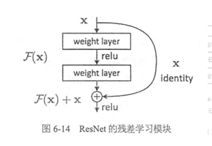
（2）模型架构

残差学习单元就是ResNet中允许原始输入信息直接传输到后层的执行机构，残差的含义就是输出-输入，所以叫做残差学习。

（3）模型特点与优势

引入残差单元的ResNet网络结构成功消除了之前的卷积神经网络中随着网络层数加深导致的测试集准确率下降的问题，随着层数的加深，ResNet在测试集上的错误率也在逐渐减小。

（4）tensorflow实现

分为三个部分，Block类用来配置残差学习模型的大小。

Block类

#50层深的ResNet使用到的Block
def resnet_v2_50(inputs,num_classes=None,global_pool=True,
                 reuse=None,scope="resnet_v2_50"):
    blocks = [
        Block("block1", residual_unit, [(256, 64, 1),(256, 64, 1),(256, 64, 2)]),
        Block("block2", residual_unit, [(512, 128, 1)] * 3 + [(512, 128, 2)]),
        Block("block3", residual_unit, [(1024, 256, 1)] * 5 + [(1024, 256, 2)]),
        Block("block4", residual_unit, [(2048, 512, 1)] * 3)]
    return resnet_v2(inputs, blocks, num_classes,reuse=reuse, scope=scope)

#101层深的ResNet使用到的Block
def resnet_v2_101(inputs,num_classes=None,global_pool=True,
                  reuse=None,scope="resnet_v2_101"):
    blocks = [
        Block("block1", residual_unit, [(256, 64, 1),(256, 64, 1),(256, 64, 2)]),
        Block("block2", residual_unit, [(512, 128, 1)] * 3 + [(512, 128, 2)]),
        Block("block3", residual_unit, [(1024, 256, 1)] * 22 + [(1024, 256, 2)]),
        Block("block4", residual_unit, [(2048, 512, 1),(2048, 512, 1),(2048, 512, 1)])]
    return resnet_v2(inputs, blocks, num_classes,reuse=reuse, scope=scope)

#200层深的ResNet使用到的Block
def resnet_v2_200(inputs,num_classes=None,global_pool=True,
                  reuse=None,scope='resnet_v2_200'):
    blocks = [
        Block("block1", bottleneck, [(256, 64, 1),(256, 64, 1),(256, 64, 2)]),
        Block("block2", bottleneck, [(512, 128, 1)] * 23 + [(512, 128, 2)]),
        Block("block3", bottleneck, [(1024, 256, 1)] * 35 + [(1024, 256, 2)]),
        Block("block4", bottleneck, [(2048, 512, 1)] * 3)]
    return resnet_v2(inputs, blocks, num_classes,reuse=reuse, scope=scope)

ResNet_struct.py 用于残差网络的搭建

import collections
import tensorflow as tf
from tensorflow.contrib import slim


class Block(collections.namedtuple("block", ["name", "residual_unit", "args"])):
    "A named tuple describing a ResNet Block"
    # namedtuple()函数原型为：
    # collections.namedtuple(typename,field_names,verbose,rename)


def conv2d_same(inputs, num_outputs, kernel_size, stride, scope=None):
    # 如果步长为1，则直接使用padding="SAME"的方式进行卷积操作
    # 一般步长不为1的情况出现在残差学习块的最后一个卷积操作中
    if stride == 1:
        return slim.conv2d(inputs, num_outputs, kernel_size, stride=1,
                           padding="SAME", scope=scope)
    else:
        pad_begin = (kernel_size - 1) // 2
        pad_end = kernel_size - 1 - pad_begin

        # pad()函数用于对矩阵进行定制填充
        # 在这里用于对inputs进行向上填充pad_begin行0，向下填充pad_end行0，
        # 向左填充pad_begin行0，向右填充pad_end行0
        inputs = tf.pad(inputs,
                        [[0, 0], [pad_begin, pad_end], [pad_begin, pad_end], [0, 0]])
        return slim.conv2d(inputs, num_outputs, kernel_size, stride=stride,
                           padding="VALID", scope=scope)


@slim.add_arg_scope
def residual_unit(inputs, depth, depth_residual, stride, outputs_collections=None,
                  scope=None):
    with tf.variable_scope(scope, "residual_v2", [inputs]) as sc:

        # 输入的通道数，取inputs的形状的最后一个元素
        depth_input = slim.utils.last_dimension(inputs.get_shape(), min_rank=4)

        # 使用slim.batch_norm()函数进行BatchNormalization操作
        preact = slim.batch_norm(inputs, activation_fn=tf.nn.relu, scope="preac")

        # 如果本块的depth值(depth参数)等于上一个块的depth(depth_input)，则考虑进行降采样操作，
        # 如果depth值不等于depth_input，则使用conv2d()函数使输入通道数和输出通道数一致
        if depth == depth_input:
            # 如果stride等于1，则不进行降采样操作，如果stride不等于1，则使用max_pool2d
            # 进行步长为stride且池化核为1x1的降采样操作
            if stride == 1:
                identity = inputs
            else:
                identity = slim.max_pool2d(inputs, [1, 1], stride=stride, scope="shortcut")
        else:
            identity = slim.conv2d(preact, depth, [1, 1], stride=stride, normalizer_fn=None,
                                   activation_fn=None, scope="shortcut")

        # 在一个残差学习块中的3个卷积层
        residual = slim.conv2d(preact, depth_residual, [1, 1], stride=1, scope="conv1")
        residual = conv2d_same(residual, depth_residual, 3, stride, scope="conv2")
        residual = slim.conv2d(residual, depth, [1, 1], stride=1, normalizer_fn=None,
                               activation_fn=None, scope="conv3")

        # 将identity的结果和residual的结果相加
        output = identity + residual

        result = slim.utils.collect_named_outputs(outputs_collections, sc.name, output)

        return result


def resnet_v2_152(inputs, num_classes, reuse=None, scope="resnet_v2_152"):
    blocks = [
        Block("block1", residual_unit, [(256, 64, 1), (256, 64, 1), (256, 64, 2)]),
        Block("block2", residual_unit, [(512, 128, 1)] * 7 + [(512, 128, 2)]),
        Block("block3", residual_unit, [(1024, 256, 1)] * 35 + [(1024, 256, 2)]),
        Block("block4", residual_unit, [(2048, 512, 1)] * 3)]
    return resnet_v2(inputs, blocks, num_classes, reuse=reuse, scope=scope)


def resnet_v2(inputs, blocks, num_classes, reuse=None, scope=None):
    with tf.variable_scope(scope, "resnet_v2", [inputs], reuse=reuse) as sc:
        end_points_collection = sc.original_name_scope + "_end_points"

        # 对函数residual_unit()的outputs_collections参数使用参数空间
        with slim.arg_scope([residual_unit], outputs_collections=end_points_collection):

            # 创建ResNet的第一个卷积层和池化层，卷积核大小7x7，深度64，池化核大侠3x3
            with slim.arg_scope([slim.conv2d], activation_fn=None, normalizer_fn=None):
                net = conv2d_same(inputs, 64, 7, stride=2, scope="conv1")
            net = slim.max_pool2d(net, [3, 3], stride=2, scope="pool1")

            # 在两个嵌套的for循环内调用residual_unit()函数堆砌ResNet的结构
            for block in blocks:
                # block.name分别为block1、block2、block3和block4
                with tf.variable_scope(block.name, "block", [net]) as sc:

                    # tuple_value为Block类的args参数中的每一个元组值，
                    # i是这些元组在每一个Block的args参数中的序号
                    for i, tuple_value in enumerate(block.args):
                        # i的值从0开始，对于第一个unit，i需要加1
                        with tf.variable_scope("unit_%d" % (i + 1), values=[net]):
                            # 每一个元组都有3个数组成，将这三个数作为参数传递到Block类的
                            # residual_unit参数中，在定义blockss时，这个参数就是函数residual_unit()
                            depth, depth_bottleneck, stride = tuple_value
                            net = block.residual_unit(net, depth=depth, depth_residual=depth_bottleneck,
                                                      stride=stride)
                    # net就是每一个块的结构
                    net = slim.utils.collect_named_outputs(end_points_collection, sc.name, net)

            # 对net使用slim.batch_norm()函数进行BatchNormalization操作
            net = slim.batch_norm(net, activation_fn=tf.nn.relu, scope="postnorm")

            # 创建全局平均池化层
            net = tf.reduce_mean(net, [1, 2], name="pool5", keep_dims=True)

            # 如果定义了num_classes，则通过1x1池化的方式获得数目为num_classes的输出
            if num_classes is not None:
                net = slim.conv2d(net, num_classes, [1, 1], activation_fn=None,
                                  normalizer_fn=None, scope="logits")

            return net

ResNet_run.py 用于残差网络的测评

import tensorflow as tf
import math
import time
import ResNet_struct
from tensorflow.contrib import slim
from datetime import datetime

batch_size = 32
num_batches = 100
num_steps_burn_in = 10
total_duration = 0.0
total_duration_squared = 0.0
inputs = tf.random_uniform((batch_size, 224, 224, 3))

def arg_scope(is_training=True,weight_decay=0.0001,batch_norm_decay=0.997,
                           batch_norm_epsilon=1e-5,batch_norm_scale=True):

    batch_norm_params = {"is_training": is_training,
                         "decay": batch_norm_decay,
                         "epsilon": batch_norm_epsilon,
                         "scale": batch_norm_scale,
                         "updates_collections": tf.GraphKeys.UPDATE_OPS}

    with slim.arg_scope([slim.conv2d],
                        #weights_initializer用于指定权重的初始化程序
                        weights_initializer=slim.variance_scaling_initializer(),
                        #weights_regularizer为权重可选的正则化程序
                        weights_regularizer=slim.l2_regularizer(weight_decay),
                        #activation_fn用于激活函数的指定，默认的为ReLU函数
                        #normalizer_params用于指定正则化函数的参数
                        activation_fn=tf.nn.relu, normalizer_fn=slim.batch_norm,
                        normalizer_params=batch_norm_params):

        #定义slim.batch_norm()函数的参数空间
        with slim.arg_scope([slim.batch_norm], **batch_norm_params):
            # slim.max_pool2d()函数的参数空间
            with slim.arg_scope([slim.max_pool2d], padding="SAME") as arg_scope:
                return arg_scope

# 定义模型的前向传播过程，这被限制在一个参数空间中
with slim.arg_scope(arg_scope(is_training=False)):
    net = ResNet_struct.resnet_v2_152(inputs, 1000)

init = tf.global_variables_initializer()
with tf.Session() as sess:
    sess.run(init)

    #运行前向传播测试过程
    for i in range(num_batches + num_steps_burn_in):
        start_time = time.time()
        _ = sess.run(net)
        duration = time.time() - start_time
        if i >= num_steps_burn_in:
            if i % 10 == 0:
                print('%s: step %d, duration = %.3f' %
                      (datetime.now(), i - num_steps_burn_in, duration))
            total_duration += duration
            total_duration_squared += duration * duration
    average_time = total_duration / num_batches

    #打印前向传播的运算时间信息
    print('%s: Forward across %d steps, %.3f +/- %.3f sec / batch' %
          (datetime.now(), num_batches, average_time,
           math.sqrt(total_duration_squared / num_batches-average_time*average_time)))


'''打印的内容
2018-04-28 15:44:25.253434: step 0, duration = 1.039
2018-04-28 15:44:35.616892: step 10, duration = 1.037
2018-04-28 15:44:45.981536: step 20, duration = 1.035
2018-04-28 15:44:56.349566: step 30, duration = 1.036
2018-04-28 15:45:06.728368: step 40, duration = 1.035
2018-04-28 15:45:17.089299: step 50, duration = 1.035
2018-04-28 15:45:27.456285: step 60, duration = 1.037
2018-04-28 15:45:37.822637: step 70, duration = 1.035
2018-04-28 15:45:48.192688: step 80, duration = 1.035
2018-04-28 15:45:58.555936: step 90, duration = 1.035
2018-04-28 15:46:07.886232: Forward across 100 steps, 1.037 +/- 0.002 sec / batch
'''