吴恩达机器学习课后作业-02逻辑回归（02-logistic_regression）

吴恩达机器学习课后作业-02逻辑回归（02-logistic_regression）

切记！！！下载第二次课后作业的题目和数据包ex2data1.txt和ex2data2.txt，数据包一定要下载，并且导入到项目所在文件夹，用Ancona或者pycharm编译都可以成功！
（后续会慢慢补充并且完善逻辑回归知识点）

一、线性可分

（案例图，假设函数，sigmoid函数y=0或y=1，损失函数，代价函数，梯度下降）
（损失函数，梯度下降函数，维度）

案例：根据学生的两门学生成绩，预测该学生是否被大学录取

数据集：ex2data1.txt

# 导入文件：
import numpy as np
import pandas as pd
import matplotlib.pyplot as plt

path = 'ex2data1.txt'
data = pd.read_csv(path,names = ['Exam 1','Exam 2','Accepted'])
data.head()

# 数据可视化：
fig,ax = plt.subplots()

ax.scatter(data[data['Accepted']==0]['Exam 1'],data[data['Accepted']==0]['Exam 2'],c = 'r',marker = 'x',label = 'y=0')
ax.scatter(data[data['Accepted']==1]['Exam 1'],data[data['Accepted']==1]['Exam 2'],c = 'b',marker = 'o',label = 'y=1')
ax.legend()

ax.set(xlabel = 'exam1',
      ylabel = 'exam2')
plt.show()

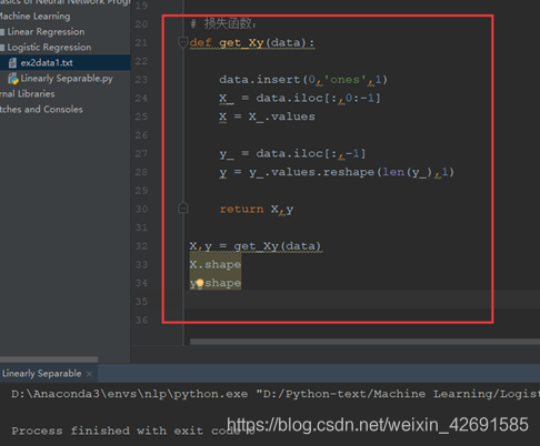
# 损失函数：
def get_Xy(data):

    data.insert(0,'ones',1)
    X_ = data.iloc[:,0:-1]
    X = X_.values

    y_ = data.iloc[:,-1]
    y = y_.values.reshape(len(y_),1)

    return X,y

X,y = get_Xy(data)
X.shape
y.shape

# 定义sigmoid函数：
def sigmoid(z):

return 1/(1 + np.exp(-z))

# 定义代价函数：
def costFunction(X,y,theta):

    A = sigmoid(X@theta)

    first = y * np.log(A)
    second = (1-y)* np.log(1 - A)

    return -np.sum (first + second)/len(X)

theta = np.zeros((3,1))
theta.shape

cost_init = costFunction(X,y,theta)
print(cost_init)

# 梯度下降：
def gradientDescent(X, y, theta, iters,alpha):
    m = len(X)
    costs = []

    for i in range(iters):
        A = sigmoid(X@theta)
        theta = theta - (alpha/m) * X.T@(A - y)
        cost = costFunction(X, y, theta)
        costs.append(cost)
        if i % 1000 == 0:
            print(cost)
    return costs,theta
alpha = 0.004
iters = 200000
costs,theta_final = gradientDescent(X,y,theta,iters,alpha)

print(theta_final)

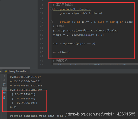
# 定义预测函数：
def predict(X, theta):

    prob = sigmoid(X @ theta)

    return [1 if x >= 0.5 else 0 for x in prob]
# 正确率：
y_ = np.array(predict(X, theta))
y_pre = y_.reshape(len(y_), 1)

acc = np.mean(y_pre == y)

print(acc)

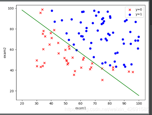
# 决策边界：
coef1 = - theta_final[0,0]/theta_final[2,0]
coef2 = - theta_final[1,0]/theta_final[2,0]

x = np.linspace(20,100,100)
f = coef1 + coef2*x

fig,ax = plt.subplots()
ax.scatter(data[data['Accepted']==0]['Exam 1'],data[data['Accepted']==0]['Exam 2'],c = 'r',marker = 'x',label = 'y=0')
ax.scatter(data[data['Accepted']==1]['Exam 1'],data[data['Accepted']==1]['Exam 2'],c = 'b',marker = 'o',label = 'y=1')
ax.legend()
ax.set(xlabel = 'exam1',
      ylabel = 'exam2')

ax.plot(x,f,c='g')
plt.show()

二、线性不可分

案例：设想你是工厂的生产主管，你要决定是否芯片要被接受或者抛弃

数据集：ex2data2.txt，芯片在两次测试中的测试结果

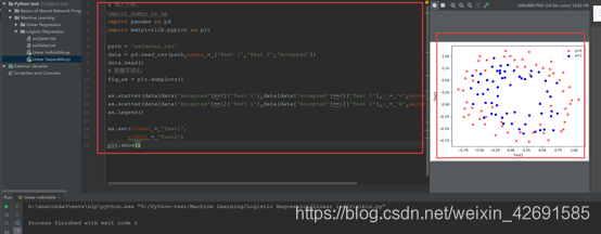
# 导入文件：
import numpy as np
import pandas as pd
import matplotlib.pyplot as plt

path = 'ex2data2.txt'
data = pd.read_csv(path,names = ['Test 1','Test 2','Accepted'])
data.head()
#数据可视化：
fig,ax = plt.subplots()

ax.scatter(data[data['Accepted']==0]['Test 1'],data[data['Accepted']==0]['Test 2'],c = 'r',marker = 'x',label = 'y=0')
ax.scatter(data[data['Accepted']==1]['Test 1'],data[data['Accepted']==1]['Test 2'],c = 'b',marker = 'o',label = 'y=1')
ax.legend()

ax.set(xlabel = 'Test1',
      ylabel = 'Test2')
plt.show()

# 特征映射：
def feature_mapping(x1,x2,power):
    data = {}

    for i in np.arange(power + 1):
        for j in np.arange(i + 1):
            data['F{}{}'.format(i - j,j)] = np.power(x1,i - j)* np.power(x2,j)

    return pd.DataFrame(data)

x1 = data['Test 1']
x2 = data['Test 2']
data2 = feature_mapping(x1,x2,6)
data2.head()

扫描二维码关注公众号，回复： 10711127 查看本文章

# 构造数据集：
X = data2.values
X.shape
y = data.iloc[:,-1].values
y = y.reshape(len(y),1)
y.shape
# 损失函数：
def sigmoid(z):
    return 1/(1 + np.exp(-z))

def costFunction(X,y,theta,lamda):
    A = sigmoid(X@theta)

    first = y*np.log(A)
    second = (1 - y)* np.log(1 - A)

    reg = np.sum(np.power(theta[1:],2)) * (lamda / (2 * len(X)))

    return  -np.sum(first + second)/len(X) + reg

theta = np.zeros((28,1))
theta.shape

lamda = 1

cost_init = costFunction(X,y,theta,lamda )
print(cost_init)

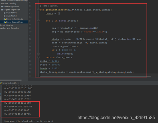
# 梯度下降函数：
def gradientDescent(X,y,theta,alpha,iters,lamda):
    costs = []

    for i in range(iters):

        reg = theta[1:] * (lamda/len(X))
        reg = np.insert(reg,0,values=0,axis=0)

        theta = theta - (X.T@(sigmoid(X@theta)- y))* alpha/len(X)-reg
        cost = costFunction(X, y, theta,lamda)
        costs.append(cost)
        if i % 1000 == 0:
            print(cost)
    return theta,costs
alpha = 0.001
iters = 200000
lamda = 0.001
theta_final,costs = gradientDescent(X,y,theta,alpha,iters,lamda)

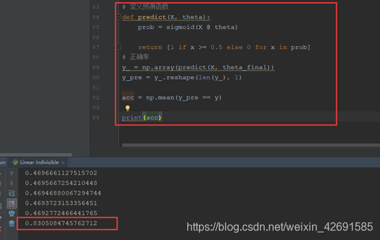
# 定义预测函数：
def predict(X, theta):
    prob = sigmoid(X @ theta)

    return [1 if x >= 0.5 else 0 for x in prob]
# 正确率：
y_ = np.array(predict(X, theta_final))
y_pre = y_.reshape(len(y_), 1)

acc = np.mean(y_pre == y)

print(acc)

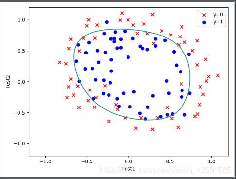
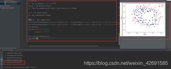
# 决策边界：
x = np.linspace(-1.2,1.2,200)
xx,yy = np.meshgrid(x,x)
z = feature_mapping(xx.ravel(),yy.ravel(),6).values

zz = z @ theta_final
zz =zz.reshape(xx.shape)

fig,ax = plt.subplots()
ax.scatter(data[data['Accepted']==0]['Test 1'],data[data['Accepted']==0]['Test 2'],c = 'r',marker = 'x',label = 'y=0')
ax.scatter(data[data['Accepted']==1]['Test 1'],data[data['Accepted']==1]['Test 2'],c = 'b',marker = 'o',label = 'y=1')
ax.legend()
ax.set(xlabel = 'Test1',
      ylabel = 'Test2')

plt.contour(xx,yy,zz,0)
plt.show()

三、附录

完整代码：

线性可分

# 导入文件：
import numpy as np
import pandas as pd
import matplotlib.pyplot as plt

path = 'ex2data1.txt'
data = pd.read_csv(path,names = ['Exam 1','Exam 2','Accepted'])
data.head()
# 数据可视化：
fig,ax = plt.subplots()

ax.scatter(data[data['Accepted']==0]['Exam 1'],data[data['Accepted']==0]['Exam 2'],c = 'r',marker = 'x',label = 'y=0')
ax.scatter(data[data['Accepted']==1]['Exam 1'],data[data['Accepted']==1]['Exam 2'],c = 'b',marker = 'o',label = 'y=1')
ax.legend()

ax.set(xlabel = 'exam1',
      ylabel = 'exam2')
plt.show()

# 损失函数：
def get_Xy(data):

    data.insert(0,'ones',1)
    X_ = data.iloc[:,0:-1]
    X = X_.values

    y_ = data.iloc[:,-1]
    y = y_.values.reshape(len(y_),1)

    return X,y

X,y = get_Xy(data)
X.shape
y.shape

# 定义sigmoid函数：
def sigmoid(z):

    return 1/(1 + np.exp(-z))
# 定义代价函数：
def costFunction(X,y,theta):

    A = sigmoid(X@theta)

    first = y * np.log(A)
    second = (1-y)* np.log(1 - A)

    return -np.sum (first + second)/len(X)

theta = np.zeros((3,1))
theta.shape

cost_init = costFunction(X,y,theta)
print(cost_init)

# 梯度下降
def gradientDescent(X, y, theta, iters,alpha):
    m = len(X)
    costs = []

    for i in range(iters):
        A = sigmoid(X@theta)
        theta = theta - (alpha/m) * X.T@(A - y)
        cost = costFunction(X, y, theta)
        costs.append(cost)
        if i % 1000 == 0:
            print(cost)
    return costs,theta
alpha = 0.004
iters = 200000
costs,theta_final = gradientDescent(X,y,theta,iters,alpha)

print(theta_final)

# 定义预测函数
def predict(X, theta):
    prob = sigmoid(X @ theta)

    return [1 if x >= 0.5 else 0 for x in prob]
# 正确率
y_ = np.array(predict(X, theta_final))
y_pre = y_.reshape(len(y_), 1)

acc = np.mean(y_pre == y)

print(acc)

# 决策边界：
coef1 = - theta_final[0,0]/theta_final[2,0]
coef2 = - theta_final[1,0]/theta_final[2,0]

x = np.linspace(20,100,100)
f = coef1 + coef2*x

fig,ax = plt.subplots()
ax.scatter(data[data['Accepted']==0]['Exam 1'],data[data['Accepted']==0]['Exam 2'],c = 'r',marker = 'x',label = 'y=0')
ax.scatter(data[data['Accepted']==1]['Exam 1'],data[data['Accepted']==1]['Exam 2'],c = 'b',marker = 'o',label = 'y=1')
ax.legend()
ax.set(xlabel = 'exam1',
      ylabel = 'exam2')

ax.plot(x,f,c='g')
plt.show()

线性不可分

# 导入文件：
import numpy as np
import pandas as pd
import matplotlib.pyplot as plt

path = 'ex2data2.txt'
data = pd.read_csv(path,names = ['Test 1','Test 2','Accepted'])
data.head()
# 数据可视化：
fig,ax = plt.subplots()

ax.scatter(data[data['Accepted']==0]['Test 1'],data[data['Accepted']==0]['Test 2'],c = 'r',marker = 'x',label = 'y=0')
ax.scatter(data[data['Accepted']==1]['Test 1'],data[data['Accepted']==1]['Test 2'],c = 'b',marker = 'o',label = 'y=1')
ax.legend()

ax.set(xlabel = 'Test1',
      ylabel = 'Test2')
plt.show()

# 特征映射：
def feature_mapping(x1,x2,power):
    data = {}

    for i in np.arange(power + 1):
        for j in np.arange(i + 1):
            data['F{}{}'.format(i - j,j)] = np.power(x1,i - j)* np.power(x2,j)

    return pd.DataFrame(data)

x1 = data['Test 1']
x2 = data['Test 2']
data2 = feature_mapping(x1,x2,6)
data2.head()

# 构造数据集:
X = data2.values
X.shape
y = data.iloc[:,-1].values
y = y.reshape(len(y),1)
y.shape
# 损失函数:
def sigmoid(z):
    return 1/(1 + np.exp(-z))

def costFunction(X,y,theta,lamda):
    A = sigmoid(X@theta)

    first = y*np.log(A)
    second = (1 - y)* np.log(1 - A)

    reg = np.sum(np.power(theta[1:],2)) * (lamda / (2 * len(X)))

    return  -np.sum(first + second)/len(X) + reg

theta = np.zeros((28,1))
theta.shape

lamda = 1

cost_init = costFunction(X,y,theta,lamda)
print(cost_init)

# 梯度下降函数：
def gradientDescent(X,y,theta,alpha,iters,lamda):
    costs = []

    for i in range(iters):

        reg = theta[1:] * (lamda/len(X))
        reg = np.insert(reg,0,values=0,axis=0)

        theta = theta - (X.T@(sigmoid(X@theta)- y))* alpha/len(X)-reg
        cost = costFunction(X, y, theta,lamda)
        costs.append(cost)
        if i % 1000 == 0:
            print(cost)
    return theta,costs
alpha = 0.001
iters = 200000
lamda = 0.001
theta_final,costs = gradientDescent(X,y,theta,alpha,iters,lamda)

# 定义预测函数
def predict(X, theta):
    prob = sigmoid(X @ theta)

    return [1 if x >= 0.5 else 0 for x in prob]
# 正确率
y_ = np.array(predict(X, theta_final))
y_pre = y_.reshape(len(y_), 1)

acc = np.mean(y_pre == y)

print(acc)

# 决策边界：
x = np.linspace(-1.2,1.2,200)
xx,yy = np.meshgrid(x,x)
z = feature_mapping(xx.ravel(),yy.ravel(),6).values

zz = z @ theta_final
zz =zz.reshape(xx.shape)

fig,ax = plt.subplots()
ax.scatter(data[data['Accepted']==0]['Test 1'],data[data['Accepted']==0]['Test 2'],c = 'r',marker = 'x',label = 'y=0')
ax.scatter(data[data['Accepted']==1]['Test 1'],data[data['Accepted']==1]['Test 2'],c = 'b',marker = 'o',label = 'y=1')
ax.legend()
ax.set(xlabel = 'Test1',
      ylabel = 'Test2')

plt.contour(xx,yy,zz,0)
plt.show()