本次进行编码的文件:
plotData.m - 绘制2D分类数据的函数
sigmoid.m - Sigmoid函数
costFunction.m - Logistic回归成本函数
predict.m - Logistic回归预测函数
costFunctionReg.m - 正则化Logistic回归成本
第一部分:逻辑回归
ex2.m(不需做改动,粘过来的原因是对新的语段进行解释)
%% Machine Learning Online Class - Exercise 2: Logistic Regression
%
% Instructions
% ------------
%
% This file contains code that helps you get started on the logistic
% regression exercise. You will need to complete the following functions
% in this exericse:
%
% sigmoid.m
% costFunction.m
% predict.m
% costFunctionReg.m
%
% For this exercise, you will not need to change any code in this file,
% or any other files other than those mentioned above.
%
%% Initialization
clear ; close all; clc
%% Load Data
% The first two columns contains the exam scores and the third column
% contains the label.
data = load('ex2data1.txt');
X = data(:, [1, 2]); y = data(:, 3);
%% ==================== Part 1: Plotting ====================
% We start the exercise by first plotting the data to understand the
% the problem we are working with.
fprintf(['Plotting data with + indicating (y = 1) examples and o ' ...
'indicating (y = 0) examples.\n']);
plotData(X, y);
% Put some labels
hold on;
% Labels and Legend
xlabel('Exam 1 score')
ylabel('Exam 2 score')
% Specified in plot order
legend('Admitted', 'Not admitted')
hold off;
fprintf('\nProgram paused. Press enter to continue.\n');
pause;
%% ============ Part 2: Compute Cost and Gradient ============
% In this part of the exercise, you will implement the cost and gradient
% for logistic regression. You neeed to complete the code in
% costFunction.m
% Setup the data matrix appropriately, and add ones for the intercept term
[m, n] = size(X);
% Add intercept term to x and X_test
X = [ones(m, 1) X];
% Initialize fitting parameters
initial_theta = zeros(n + 1, 1);
% Compute and display initial cost and gradient
[cost, grad] = costFunction(initial_theta, X, y);
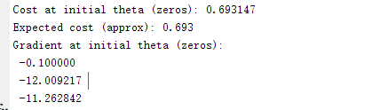
fprintf('Cost at initial theta (zeros): %f\n', cost);
fprintf('Expected cost (approx): 0.693\n');
fprintf('Gradient at initial theta (zeros): \n');
fprintf(' %f \n', grad);
fprintf('Expected gradients (approx):\n -0.1000\n -12.0092\n -11.2628\n');
% Compute and display cost and gradient with non-zero theta
test_theta = [-24; 0.2; 0.2];
[cost, grad] = costFunction(test_theta, X, y);
fprintf('\nCost at test theta: %f\n', cost);
fprintf('Expected cost (approx): 0.218\n');
fprintf('Gradient at test theta: \n');
fprintf(' %f \n', grad);
fprintf('Expected gradients (approx):\n 0.043\n 2.566\n 2.647\n');
fprintf('\nProgram paused. Press enter to continue.\n');
pause;
%% ============= Part 3: Optimizing using fminunc =============
% In this exercise, you will use a built-in function (fminunc) to find the
% optimal parameters theta.
% Set options for fminunc
options = optimset('GradObj', 'on', 'MaxIter', 400);%GradObj 设置为on ,告诉fminunc 函数返回成本和渐变,迭代次数400
% Run fminunc to obtain the optimal theta (获得最佳θ)
% This function will return theta and the cost
[theta, cost] = ...
fminunc(@(t)(costFunction(t, X, y)), initial_theta, options);%@(t)(costFunction(t, X, y)),所需求解最小值的代价函数,@为函数句柄,@后面括号里的 t 表示函数的参数,也就是我们所需要求解最小代价的参数θ
% Print theta to screen
fprintf('Cost at theta found by fminunc: %f\n', cost);
fprintf('Expected cost (approx): 0.203\n');
fprintf('theta: \n');
fprintf(' %f \n', theta);
fprintf('Expected theta (approx):\n');
fprintf(' -25.161\n 0.206\n 0.201\n');
% Plot Boundary
plotDecisionBoundary(theta, X, y);
% Put some labels
hold on;
% Labels and Legend
xlabel('Exam 1 score')
ylabel('Exam 2 score')
% Specified in plot order
legend('Admitted', 'Not admitted')
hold off;
fprintf('\nProgram paused. Press enter to continue.\n');
pause;
%% ============== Part 4: Predict and Accuracies ==============
% After learning the parameters, you'll like to use it to predict the outcomes
% on unseen data. In this part, you will use the logistic regression model
% to predict the probability that a student with score 45 on exam 1 and
% score 85 on exam 2 will be admitted.
%
% Furthermore, you will compute the training and test set accuracies of
% our model.
%
% Your task is to complete the code in predict.m
% Predict probability for a student with score 45 on exam 1
% and score 85 on exam 2
prob = sigmoid([1 45 85] * theta);
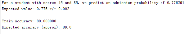
fprintf(['For a student with scores 45 and 85, we predict an admission ' ...
'probability of %f\n'], prob);
fprintf('Expected value: 0.775 +/- 0.002\n\n');
% Compute accuracy on our training set
p = predict(theta, X);
fprintf('Train Accuracy: %f\n', mean(double(p == y)) * 100);
fprintf('Expected accuracy (approx): 89.0\n');
fprintf('\n');
1.PlotData.m
function plotData(X, y)
%PLOTDATA Plots the data points X and y into a new figure
%   PLOTDATA(x,y) plots the data points with + for the positive examples
%   and o for the negative examples. X is assumed to be a Mx2 matrix.

% Create New Figure
figure; hold on;

% ====================== YOUR CODE HERE ======================
% Instructions: Plot the positive and negative examples on a
%               2D plot, using the option 'k+' for the positive
%               examples and 'ko' for the negative examples.
%
% Find Indices of Positive and Negative Examples
 pos = find(y==1); neg = find(y == 0);  %查找该元素的索引和值

% Plot Examples
plot(X(pos, 1), X(pos, 2), 'k+','LineWidth', 2,'MarkerSize', 7);
plot(X(neg, 1), X(neg, 2), 'ko', 'MarkerFaceColor', 'y','MarkerSize', 7);%y是黄色的意思哦……

% =========================================================================

hold off;

end
2.Sigmoid.m
function g = sigmoid(z)
%SIGMOID Compute sigmoid function
%   g = SIGMOID(z) computes the sigmoid of z.

% You need to return the following variables correctly
g = zeros(size(z));%创建全0数组

% ====================== YOUR CODE HERE ======================
% Instructions: Compute the sigmoid of each value of z (z can be a matrix,
%               vector or scalar).

g = 1 ./ ( 1 + exp(-z) ) ;  %1./x表示矩阵中每一个元素的倒数,exp,以自然常数e为底的指数函数

% =============================================================

end
3.CostFunction.m
实现逻辑回归的成本函数和梯度。
完成costFunction.m中的代码以返回成本和渐变。
MATLAB关于costfunction的解释:
costFunction Compute cost and gradient for logistic regression
J = costFunction(theta, X, y) computes the cost of using theta as the
parameter for logistic regression and the gradient of the cost
w.r.t. to the parameters.
function [J, grad] = costFunction(theta, X, y)  %gray英文gradient的缩写
%COSTFUNCTION Compute cost and gradient for logistic regression
%   J = COSTFUNCTION(theta, X, y) computes the cost of using theta as the
%   parameter for logistic regression and the gradient of the cost
%   w.r.t. to the parameters.

% Initialize some useful values
m = length(y); % number of training examples

% You need to return the following variables correctly
J = 0;
grad = zeros(size(theta));

% ====================== YOUR CODE HERE ======================
% Instructions: Compute the cost of a particular choice of theta.
%               You should set J to the cost.
%               Compute the partial derivatives and set grad to the partial
%               derivatives of the cost w.r.t. each parameter in theta
%
% Note: grad should have the same dimensions as theta
%
J = 1/m*(-y'*log(sigmoid(X*theta)) - (1-y)'*(log(1-sigmoid(X*theta))));
grad = 1/m * X'*(sigmoid(X*theta) - y);

% =============================================================

end
4.使用fminunc 学习参数
options = optimset('GradObj', 'on', 'MaxIter', 400);   %GradObj 设置为on ,告诉fminunc 函数返回成本和渐变,迭代次数400


[theta, cost] = ...
	fminunc(@(t)(costFunction(t, X, y)), initial_theta, options);
@是Matlab中的句柄函数的标志符,即间接的函数调用方法。
@后面括号里的 t 表示函数的参数,也就是我们所需要求解最小代价的参数θ,最后一部分为匿名函数的表达式。

具体关于句柄表示去看这位博主的原创(上面这张截图也是来自这位大大) http://blog.csdn.net/yhl_leo/article/details/50699990

5.predict.m
输入X和theta,返回预测结果向量。每个值是 0 或 1 ;
round函数:四舍五入到最近整数
function p = predict(theta, X)
%PREDICT Predict whether the label is 0 or 1 using learned logistic
%regression parameters theta
%   p = PREDICT(theta, X) computes the predictions for X using a
%   threshold at 0.5 (i.e., if sigmoid(theta'*x) >= 0.5, predict 1)

m = size(X, 1); % Number of training examples

% You need to return the following variables correctly
p = zeros(m, 1);   %m行1列

% ====================== YOUR CODE HERE ======================
% Instructions: Complete the following code to make predictions using
%               your learned logistic regression parameters.
%               You should set p to a vector of 0's and 1's

p = round(sigmoid(X * theta));

% =========================================================================
end
如一个学生成绩为45与85,使用这个逻辑回归模型得出他被录取的概率为0.776
第二部分:正则化逻辑回归
%% Machine Learning Online Class - Exercise 2: Logistic Regression
%
% Instructions
% ------------
%
% This file contains code that helps you get started on the second part
% of the exercise which covers regularization with logistic regression.
%
% You will need to complete the following functions in this exericse:
%
% sigmoid.m
% costFunction.m
% predict.m
% costFunctionReg.m
%
% For this exercise, you will not need to change any code in this file,
% or any other files other than those mentioned above.
%
%% Initialization
clear ; close all; clc
%% Load Data
% The first two columns contains the X values and the third column
% contains the label (y).
data = load('ex2data2.txt');
X = data(:, [1, 2]); y = data(:, 3);
plotData(X, y);
% Put some labels
hold on;
% Labels and Legend
xlabel('Microchip Test 1')
ylabel('Microchip Test 2')
% Specified in plot order
legend('y = 1', 'y = 0')
hold off;
%% =========== Part 1: Regularized Logistic Regression ============
% In this part, you are given a dataset with data points that are not
% linearly separable. However, you would still like to use logistic
% regression to classify the data points.
%
% To do so, you introduce more features to use -- in particular, you add
% polynomial features to our data matrix (similar to polynomial
% regression).
%
% Add Polynomial Features(多项式特征)
% Note that mapFeature also adds a column of ones for us, so the intercept
% term is handled
X = mapFeature(X(:,1), X(:,2))%调用下面的mapFeature.m文件中的mapFeature(X1,X2)函数
%将只有x1,x2feature map成一个有28个feature的6次的多项式 ,这样就能画出更复杂的decision boundary, 但同时也有可能带来overfitting的结果(取决于λ的值)
%调用完后X变为118*28(118个example,28个属性,包括前面的1做为一列)的矩阵;
% Initialize fitting parameters
initial_theta = zeros(size(X, 2), 1);
% Set regularization parameter lambda to 1
lambda = 1;% λ=1;当λ=0时表示不正则化(No regularization ),这时会出现overfitting;当λ=100时会出现Too much regularization(Underfitting)
% Compute and display initial cost and gradient for regularized logistic
% regression
[cost, grad] = costFunctionReg(initial_theta, X, y, lambda);%调用costFunctionReg.m文件中的costFunctionReg(theta, X, y, lambda)函数
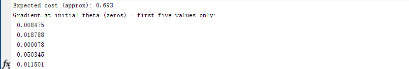
fprintf('Cost at initial theta (zeros): %f\n', cost);%计算initial theta (zeros)时的cost 值
fprintf('Expected cost (approx): 0.693\n');
fprintf('Gradient at initial theta (zeros) - first five values only:\n');
fprintf(' %f \n', grad(1:5));
fprintf('Expected gradients (approx) - first five values only:\n');
fprintf(' 0.0085\n 0.0188\n 0.0001\n 0.0503\n 0.0115\n');
fprintf('\nProgram paused. Press enter to continue.\n');
pause;
% Compute and display cost and gradient
% with all-ones theta and lambda = 10
test_theta = ones(size(X,2),1);%生成一个与X列相同的矩阵,元素都为1
[cost, grad] = costFunctionReg(test_theta, X, y, 10);%lamda=10
fprintf('\nCost at test theta (with lambda = 10): %f\n', cost);
fprintf('Expected cost (approx): 3.16\n');
fprintf('Gradient at test theta - first five values only:\n');
fprintf(' %f \n', grad(1:5));
fprintf('Expected gradients (approx) - first five values only:\n');
fprintf(' 0.3460\n 0.1614\n 0.1948\n 0.2269\n 0.0922\n');
fprintf('\nProgram paused. Press enter to continue.\n');
pause;
%% ============= Part 2: Regularization and Accuracies =============
% Optional Exercise:
% In this part, you will get to try different values of lambda and
% see how regularization affects the decision coundart
%
% Try the following values of lambda (0, 1, 10, 100).
%
% How does the decision boundary change when you vary lambda? How does
% the training set accuracy vary?
%
% Initialize fitting parameters
initial_theta = zeros(size(X, 2), 1);
% Set regularization parameter lambda to 1 (you should vary this)
lambda = 1;
% Set Options
options = optimset('GradObj', 'on', 'MaxIter', 400);
% Optimize
[theta, J, exit_flag] = ...
fminunc(@(t)(costFunctionReg(t, X, y, lambda)), initial_theta, options);
% Plot Boundary
plotDecisionBoundary(theta, X, y);
hold on;
title(sprintf('lambda = %g', lambda))
% Labels and Legend
xlabel('Microchip Test 1')
ylabel('Microchip Test 2')
legend('y = 1', 'y = 0', 'Decision boundary')
hold off;
% Compute accuracy on our training set
p = predict(theta, X);
fprintf('Train Accuracy: %f\n', mean(double(p == y)) * 100);
fprintf('Expected accuracy (with lambda = 1): 83.1 (approx)\n');
1.mapFeature.m
特征映射 没有改动,就是一段生成x1,x2,x1^2,etc……代码。
function out = mapFeature(X1, X2)
% MAPFEATURE Feature mapping function to polynomial features
%
%   MAPFEATURE(X1, X2) maps the two input features
%   to quadratic features used in the regularization exercise.
%
%   Returns a new feature array with more features, comprising of
%   X1, X2, X1.^2, X2.^2, X1*X2, X1*X2.^2, etc..
%
%   Inputs X1, X2 must be the same size
%

degree = 6;
out = ones(size(X1(:,1)));
for i = 1:degree   %i从1到6
    for j = 0:i    %j从0到i
        out(:, end+1) = (X1.^(i-j)).*(X2.^j);
    end
end

end
2.costfunction.m
function [J, grad] = costFunctionReg(theta, X, y, lambda)
%COSTFUNCTIONREG Compute cost and gradient for logistic regression with regularization
%   J = COSTFUNCTIONREG(theta, X, y, lambda) computes the cost of using
%   theta as the parameter for regularized logistic regression and the
%   gradient of the cost w.r.t. to the parameters.

% Initialize some useful values
m = length(y); % number of training examples

% You need to return the following variables correctly
J = 0;
grad = zeros(size(theta));

% ====================== YOUR CODE HERE ======================
% Instructions: Compute the cost of a particular choice of theta.
%               You should set J to the cost.
%               Compute the partial derivatives and set grad to the partial
%               derivatives of the cost w.r.t. each parameter in theta

J = 1/m * sum(-y' * log(sigmoid(X*theta)) - (1 - y') * log(1 - sigmoid(X * theta))) + lambda/2/m*sum(theta(2:end).^2);

grad(1,:) = 1/m * (X(:, 1)' * (sigmoid(X*theta) - y));
grad(2:size(theta), :) = 1/m * (X(:, 2:size(theta))' * (sigmoid(X*theta) - y))...
        + lambda/m*theta(2:size(theta), :);
% =============================================================

end
3.plotDecisionBoundary.m
代码没有进行改动 ,理解一下 (还是没看懂)
通过在均匀间隔的网格上计算分类器的预测来绘制非线性决策边界,然后绘制预测从y = 0变为y = 1 的轮廓图
function plotDecisionBoundary(theta, X, y)
%PLOTDECISIONBOUNDARY Plots the data points X and y into a new figure with
%the decision boundary defined by theta
%   PLOTDECISIONBOUNDARY(theta, X,y) plots the data points with + for the
%   positive examples and o for the negative examples. X is assumed to be
%   a either
%   1) Mx3 matrix, where the first column is an all-ones column for the
%      intercept.
%   2) MxN, N>3 matrix, where the first column is all-ones

% Plot Data
plotData(X(:,2:3), y);%取第2 3列
hold on

if size(X, 2) <= 3 %列数小于等于3
    % Only need 2 points to define a line, so choose two endpoints
    % decision boundary为一条直线,画直线只需要两点就可以
    plot_x = [min(X(:,2))-2,  max(X(:,2))+2];

    % Calculate the decision boundary line%求plot_y(x2)
    % 矩阵和标量相加减(theta(2).*plot_x + theta(1))实质是矩阵每个元素与该标量相加减
    plot_y = (-1./theta(3)).*(theta(2).*plot_x + theta(1));

    % Plot, and adjust axes for better viewing
    plot(plot_x, plot_y)

    % Legend, specific for the exercise
    legend('Admitted', 'Not admitted', 'Decision Boundary')
    axis([30, 100, 30, 100])%axis - 设置轴范围和纵横比
else
    % Here is the grid range
    u = linspace(-1, 1.5, 50);
    v = linspace(-1, 1.5, 50);

    z = zeros(length(u), length(v));
    % Evaluate z = theta*x over the grid
    for i = 1:length(u)
        for j = 1:length(v)
            z(i,j) = mapFeature(u(i), v(j))*theta;
        end
    end
    z = z'; % important to transpose z before calling contour

    % Plot z = 0
    % Notice you need to specify the range [0, 0]
    contour(u, v, z, [0, 0], 'LineWidth', 2)
end
hold off

end
使用正则化之后的图
