文|Seraph
00 | 绪论:初识机器学习
Welcome
- 生活中常见的机器学习使用场景
- google搜索页面排序
- 苹果相册自动识别朋友图片
- 垃圾邮件过滤
- 不仅要学习机器学习算法含义,还要想怎么将算法应用到我们生活中的场景。平常多思考怎么利用机器学习算法解决我们工作中遇到的问题。
- 应用领域
- Database mining
E.g.,Web click data, medical records, bilolgy, engineering - Applicatins cant program by hand
E.g.,Autonomours helicopter, handwriting recognition, most of Natural Language Processing, Computer Vision. - Self-customizing programs
E.g.,Amazon, Netflix product recommendations - Understanding human learning(brain, real AI).
What is machine learning
- Machine Learning definition
- Arthur Samuel(1959). Machine Learning: Field of study that gives computers the ability to learn without being explicitly programmed.
- Tom Mitchell(1998). Well-posed Learning Problem: A computer program is said to learn from experience E with respect to some task T and some performance measure P, if its performance on T, as measured by P, imporves with experience E.
Example: playing checkers.
E = the experience of playing many games of checkers
T = the task of playing checkers.
P = the probability that the program will win the next game.
- Machine learning algorithms:
- Supervised learning
- Unsupervised learning
Others: Reinforcement learning, recommender systems.
- Practical advice for applying learning algorithms.
解决什么问题,用什么算法比较适合,这个可以说是一个算法工程师最为重要的能力。也是区别算法工程师的能力的关键所在。
Supervised Learning
- Supervised Learning: “right answers” given.
- Regression: Predict continuous valued output.
- Classification: Discrete valued output.
Unsupervised Learning
1.使用场景
- Google News
- Genes
- Organize computing clusters
- Social network analysis
- Market segmentation
- Astronomical data analysis
- Cocktail party problem
algorithm:
01 | Linear regression with one variable
Model representation

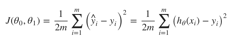
Cost function
Gradient descent
-
因为梯度下降法不能确定是全局最优,所有我们经常给不同的参数初始值来重复做实验。这样可能得到的结果不一样。
但是对于凸函数来说,是能保证全局最优的。

-
注意所有参数值要同步更新

-
学习率与收敛的关系

-
“Batch” Gradient Descent
“Batch”: Each step of gradient descentuses all the training examples. -
即使固定的学习率,梯度下降也能收敛到局部最小值。

02 | Linear Algebra review
Matrices and Vectors
- Matrices are not commutative: A∗B≠B∗A
- Matrices are associative: (A∗B)∗C=A∗(B∗C)
- 注意以下单位矩阵的维数不一样

03 | Environment Setupe Instructions
04 | Multivariate Linear Regression
Multiple Features
- 将 x 0 = 1 x_0=1 x0=1,形成m+1的特征。

- 特征缩放:统一特征权重、使梯度下降算法更快地收敛。(相近即可,不一定要范围完全一致)

- Min-Max normalization
x ′ = x − m i n ( x ) m a x ( x ) − m i n ( x ) x^ {'}=\frac{x-min(x)}{max(x)-min(x)} x′=max(x)−min(x)x−min(x) - Mean normalization
x ′ = x − a v e r a g e ( x ) m a x ( x ) − m i n ( x ) x^{'}=\frac{x-average(x)}{max(x)-min(x)} x′=max(x)−min(x)x−average(x) - standardization / z-score normalization
x ′ = x − x ˉ σ x^{'}=\frac{x-\bar{x}}{\sigma} x′=σx−xˉ - max abs normalization
x ′ = x ∣ ∣ m a x ( x ) ∣ ∣ x^{'}=\frac{x}{||max(x)||} x′=∣∣max(x)∣∣x - robust normalization(先减去中位数,再除以四分位间距(interquartile range))
x ′ = x − m e d i a n ( x ) I Q R ( x ) x^{'}=\frac{x-median(x)}{IQR(x)} x′=IQR(x)x−median(x)
Features and Polynomial Regression
- 多项式的特征需要进行缩放。

03 | Computing Parameters Analytically
Normal Equation
θ = ( X T X ) − 1 X T y \theta=(X^TX)^{-1}X^Ty θ=(XTX)−1XTy
- 梯度下降与正规方程对比

- 使用正规方式,就不需要对特征进行缩放了。
- 当feature少时,使用Normal Equation比较好;当features多的时候,使用Gradient Descent比较好。
虽然Normal Equation不需要迭代、不需要指定学习率,但是其计算复杂度高,计算矩阵的逆需要n的3次方。 - 当使用更复杂的分类模型,如逻辑回归,正规方程就不适用了。
- Normal Equation Noninvertibility

- 奇异或退化矩阵(singular or degenerate matrices)
- pinv(pseudo-inverse)伪逆:即使矩阵不存在逆的情况下,该函数也会返回逆。
05 | Octave Tutorial
Basic operations
1~= 2中的~表示不等于。- %表示注释
xor(1, 0)中的xor表示异或PS1('>> ')该表输入提示符。a = 3;加;可以阻止打印disp(a)表示显示。disp(sprintf('2 decimals: %0.2f', a))format long改变输出默认长度为longv = [1 2 3]表示行向量生成方式v=[1; 2; 3]表示列向量生成方式v=1:0.1:2表示从1到2,步长为0.1生成行向量。(步长默认为1)one(2, 3)表示生成2x3的都为1的矩阵。同类型:zeros(2, 3),随机矩阵rand(2, 3),高斯分布矩阵randn(2, 3),单位矩阵eye(2, 3)hist(w)表示绘制直方图help eye表示查询相关指令信息
Moving data around
- size
size(a)表示矩阵维度,返回的是1xN的矩阵。
size(a, 1)表示矩阵第1维度。 - length
length(a)表示矩阵最长的维度。 load('featureX.dat')表示载入文件数据。who表示显示当前作用域内所有变量。whos表示显示当前作用域内所有变量详细情况(维度、占用空间、类型)。clear a表示清楚变量a。v = a(1:10)表示将a矩阵的1~10行数据赋给v。save v.mat v表示保存v矩阵到v.mat文件中
save hello.txt v -ascii表示以ascii码的形式存储数据,默认是以二进制的形式。A(:,2) = [10; 11; 12]表示A矩阵第2列换成[10; 11; 12],注意A矩阵被改变了。A = [A, [100; 101; 102]]表示A矩阵增加一列[100; 101; 102]。A(:)表示取出A矩阵中所有的值成一个向量。C = [A B]表示A矩阵和B矩阵横向合并成C矩阵。
D = [A; B]表示A矩阵和B矩阵纵向合并成D矩阵。
Computing on Data
A*B表示矩阵的乘法。A.*B表示矩阵的点积。
A.^2表示对矩阵A的所有元素进行平方计算。
1./A表示对矩阵A的所有元素进行求倒数计算。
以上公式中的.表示对矩阵元素进行操作。- 对数
log(A),e指数exp(A),绝对值abs(A),负数-A。 A+1表示矩阵A所有元素加+1。A'表示矩阵A的转置。[val, ind] = max(a)表示如果a是向量,返回向量的最大值及相应位置;
如果a是矩阵,则返回每一列的最大值及相应位置。A < 3表示返回小于3的布尔矩阵。find(A < 3)表示找到矩阵A中小于3的元素的位置。(按列读取)
[r, c] = find(A <3)表示找到矩阵A中小于3的元素行列位置。magic(3)表示生成3x3的幻方矩阵。(任意行、列、对角线相加和相等)- 求和
sum(a),求乘积prod(a),向下取整floor(a),向上取整ceil(a)。 max(A, [], 1)表示矩阵A每列的最大值,max(A)默认取每列的最大值。
max(A, [], 2)表示矩阵A每行的最大值。max(max(a)或者max(a(:))表示求矩阵a的最大值。- 部分函数的参数用1表示列,2表示行。
sum(sum(A .*eye(lenght(A))))表示求A对象线的和。(A为MxM维度)flipud(A)表示使矩阵A垂直翻转。
Plotting data
plot(x, y, 'r')表示以x,y为横纵坐标用红色线进行画图。hold on表示保持住之前的绘画。xlabel('time')表示标注横坐标为time。ylable('value)`表示标注纵坐标为value。legend('sin', 'cos')表示标注线的标识。title('my plot)`表示标准标题为my plot。print -dpng 'myplot.png'表示将绘图打印成PNG图片保存。close表示关闭绘图显示。figure(1); plot(t, y1)表示在figure1中绘图。subplot(1, 2, 1)表示将画板分层1行2列,使用第1个进行绘画。axis([x1 x2 y1 y2])表示设置绘图的横纵坐标的范围。clf表示清理绘图。imagesc(A), colorbar, colormap gray;表示用色块显示矩阵。
Control Statements
- for语法
for i=1:10,
	v(i) = 2^i;
end;
- while语法
while i <= 5,
	v(i) = 100;
	i = i+1;
end;
- if语法
if v(1)==1,
	disp('1');
elseif v(2)==2,
	disp("2");
else
	disp("3");
end;
- 函数
function [y1, y2] = squareAndCubeThisNumber(x)
	y1 = x^2;
	y2 = x^3;
文件名要和函数名一致,否则其它文件无法导入。
-
添加搜索路径
addpaht('/Path') -
代价函数
function J = costFunctionJ(X, y, theta)
	m = size(X, 1);
	predictions = X*theta;
	sqrErrors = (predictions-y).^2;
	J = 1/(2*m)*sum(sqrErrors);
Vectorization

06 | Logistic回归
Classifer
- 通常使用线性回归进行分类不是个好方法。如下额外的一个样本,导致整体分类效果差很多。

逻辑回归可以将输出结果限制到[0, 1]。Logistic Regression是一种分类算法,而不是回归算法。

Hypothesis Representation
- Sigmoid function 与 Logistic function是同义词。