作业二:ex2答案解析
一、逻辑回归
第一部分:
ex2.m文件代码解读:
clear ;
close all;
clc;
data = load('ex2data1.txt'); %读取数据
X = data(:, [1, 2]); y = data(:, 3); %data是一个矩阵,X为第一到第二列所有的行的值组成一个矩阵
plotData(X, y); %调用函数(筛选的数据、画图的规则)
hold on;
%两个轴的名称
xlabel('Exam 1 score');
ylabel('Exam 2 score');
%标记符号所对应的名称,按先后顺序,即:加号是Admitted,圆圈是Not admitted,标记在图的右上角
legend('Admitted', 'Not admitted')
hold off;
fprintf('\nProgram paused. Press enter to continue.\n');%按压任意键继续
pause; %程序暂停
[m, n] = size(X); %m行n列
X = [ones(m, 1) X]; %m行一列的元素全为1向量
initial_theta = zeros(n + 1, 1);%初始化theta,都为0
%计算并显示初始成本和梯度
[cost, grad] = costFunction(initial_theta, X, y); %调用函数
fprintf('Cost at initial theta (zeros): %f\n', cost); %打印代价
fprintf('Expected cost (approx): 0.693\n');
fprintf('Gradient at initial theta (zeros): \n');
fprintf(' %f \n', grad); %打印梯度
fprintf('Expected gradients (approx):\n -0.1000\n -12.0092\n -11.2628\n');
%使用非零θ计算和显示成本和梯度
test_theta = [-24; 0.2; 0.2];
[cost, grad] = costFunction(test_theta, X, y);
fprintf('\nCost at test theta: %f\n', cost);
fprintf('Expected cost (approx): 0.218\n');
fprintf('Gradient at test theta: \n');
fprintf(' %f \n', grad);
fprintf('Expected gradients (approx):\n 0.043\n 2.566\n 2.647\n');
fprintf('\nProgram paused. Press enter to continue.\n');
pause;
%用内置函数找最佳参数theta
%?'GradObj','on':用户自己定义函数的梯度。
%?'MaxIter',400:允许的最大迭代次数为400
options = optimset('GradObj', 'on', 'MaxIter', 400);
%fminuc函数的作用为取最小值
%theta和代价
[theta, cost] = fminunc(@(t)(costFunction(t, X, y)), initial_theta, options);
%打印theta
fprintf('Cost at theta found by fminunc: %f\n', cost);
fprintf('Expected cost (approx): 0.203\n');
fprintf('theta: \n');
fprintf(' %f \n', theta);
fprintf('Expected theta (approx):\n');
fprintf(' -25.161\n 0.206\n 0.201\n');
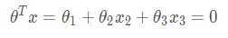
%画出决策边界
plotDecisionBoundary(theta, X, y);
hold on;
xlabel('Exam 1 score')
ylabel('Exam 2 score')
legend('Admitted', 'Not admitted')
hold off;
fprintf('\nProgram paused. Press enter to continue.\n');
pause;
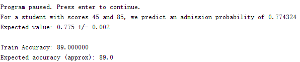
%预测和准确性
prob = sigmoid([1 45 85] * theta);
fprintf('For a student with scores 45 and 85, we predict an admission probability of %f\n', prob);
fprintf('Expected value: 0.775 +/- 0.002\n\n');
p = predict(theta, X);
fprintf('Train Accuracy: %f\n', mean(double(p == y)) * 100); %训练精确度
fprintf('Expected accuracy (approx): 89.0\n'); %期待的结果
fprintf('\n');
第二部分:
plotData.m文件代码解读:
function plotData(X,y)
figure;
hold on;
% 寻找1和0的项
pos = find(y == 1); neg = find(y == 0);
% 画图
plot(X(pos, 1), X(pos, 2), 'k+','LineWidth', 2, 'MarkerSize', 7);
plot(X(neg, 1), X(neg, 2), 'ko', 'MarkerFaceColor', 'y','MarkerSize', 7);
hold off;
end
注意:
plot函数用法:https://blog.csdn.net/qq_43211132/article/details/88235315
find函数用法:
https://blog.csdn.net/qq_43211132/article/details/88236920
执行结果:

第三部分
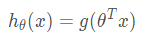
sigmoid.m文件代码解读
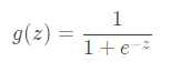
hypothesis函数定义为
function g = sigmoid(z)
g = zeros(size(z));%初始化g
g = 1 ./ ( 1 + exp(-z) ) ;
end
第四部分
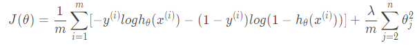
costFunction.m文件代码解读
逻辑回归似然函数取对数为:
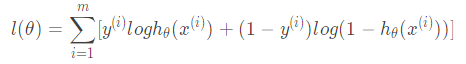
要想取得最大似然估计,可令代价函数为:
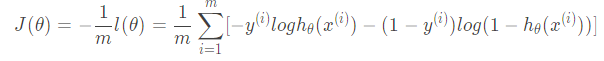
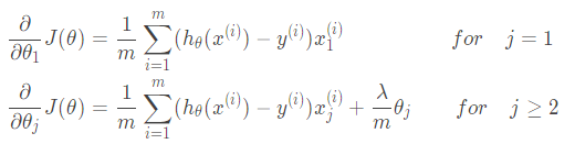
求导得

function [J, grad] = costFunction(theta, X, y)
m = length(y);%m为训练样本的数目
%初始化J和grad
J = 0;
grad = zeros(size(theta));
J= -1 * sum( y .* log( sigmoid(X*theta) ) + (1 - y ) .* log( (1 - sigmoid(X*theta)) ) ) / m ;
grad = ( X' * (sigmoid(X*theta) - y ) )/ m ;
end
运行结果:

第五部分:
fminunc()函数,见第一部分中间;
%fminuc函数的作用为取最小值
%theta和代价
[theta, cost] = fminunc(@(t)(costFunction(t, X, y)), initial_theta, options);
%打印theta
fprintf('Cost at theta found by fminunc: %f\n', cost);
fprintf('Expected cost (approx): 0.203\n');
fprintf('theta: \n');
fprintf(' %f \n', theta);
fprintf('Expected theta (approx):\n');
fprintf(' -25.161\n 0.206\n 0.201\n');
运行结果:

第六部分
plotDecisionBoundary.m:画决策边界
function plotDecisionBoundary(theta, X, y)
%X为m*3的矩阵了,第一列为1,现取第二列第三列加上y作图
plotData(X(:,2:3), y);
hold on
if size(X, 2) <= 3
    % 选两个点确定一条直线
    plot_x = [min(X(:,2))-2,  max(X(:,2))+2];

    % 计算决策边界线
    plot_y = (-1./theta(3)).*(theta(2).*plot_x + theta(1));

    % 绘制坐标
    plot(plot_x, plot_y)

    %标记符号所对应的名称,按先后顺序
    legend('Admitted', 'Not admitted', 'Decision Boundary')
    axis([30, 100, 30, 100]) %设置坐标范围,axis([xmin xmax ymin ymax])
else
    % 网格范围,头为-1,尾为1.5,共有50各元素,每个元素等距
    u = linspace(-1, 1.5, 50);
    v = linspace(-1, 1.5, 50);

    z = zeros(length(u), length(v));
    % 在网格上评估 z = theta*x
    for i = 1:length(u)
        for j = 1:length(v)
            z(i,j) = mapFeature(u(i), v(j))*theta;
        end
    end
    z = z'; % 在调用轮廓之前转置z很重要

    % contour(u,v,z,n)是画等值线
    contour(u, v, z, [0, 0], 'LineWidth', 2)
end
hold off

end
运行结果

第七部分
predict.m:计算模型精确度
function p = predict(theta, X)
m = size(X, 1);
%初始化p
p = zeros(m, 1);
%先计算预测值
k = find(sigmoid( X * theta) >= 0.5 );
p(k)= 1;
d = find(sigmoid( X * theta) < 0.5 );
p(d)= 0;
end
运行结果:
二、逻辑回归(多项式回归)
er2_reg.m
clear ;
close all;
clc
data = load('ex2data2.txt');
X = data(:, [1, 2]);
y = data(:, 3);
plotData(X, y);
hold on;
xlabel('Microchip Test 1')
ylabel('Microchip Test 2')
legend('y = 1', 'y = 0')
hold off;
%第一部分:规范化Logistic回归
X = mapFeature(X(:,1), X(:,2));
initial_theta = zeros(size(X, 2), 1);
lambda = 1;
[cost, grad] = costFunctionReg(initial_theta, X, y, lambda);

fprintf('Cost at initial theta (zeros): %f\n', cost);
fprintf('Expected cost (approx): 0.693\n');
fprintf('Gradient at initial theta (zeros) - first five values only:\n');
fprintf(' %f \n', grad(1:5));
fprintf('Expected gradients (approx) - first five values only:\n');
fprintf(' 0.0085\n 0.0188\n 0.0001\n 0.0503\n 0.0115\n');

fprintf('\nProgram paused. Press enter to continue.\n');
pause;

test_theta = ones(size(X,2),1);
[cost, grad] = costFunctionReg(test_theta, X, y, 10);

fprintf('\nCost at test theta (with lambda = 10): %f\n', cost);
fprintf('Expected cost (approx): 3.16\n');
fprintf('Gradient at test theta - first five values only:\n');
fprintf(' %f \n', grad(1:5));
fprintf('Expected gradients (approx) - first five values only:\n');
fprintf(' 0.3460\n 0.1614\n 0.1948\n 0.2269\n 0.0922\n');

fprintf('\nProgram paused. Press enter to continue.\n');
pause;

%正规化和准确性
initial_theta = zeros(size(X, 2), 1);
lambda = 1;
options = optimset('GradObj', 'on', 'MaxIter', 400);
[theta, J, exit_flag] = fminunc(@(t)(costFunctionReg(t, X, y, lambda)), initial_theta, options);
plotDecisionBoundary(theta, X, y);
hold on;
title(sprintf('lambda = %g', lambda))

xlabel('Microchip Test 1')
ylabel('Microchip Test 2')

legend('y = 1', 'y = 0', 'Decision boundary')
hold off;
p = predict(theta, X);

fprintf('Train Accuracy: %f\n', mean(double(p == y)) * 100);
fprintf('Expected accuracy (with lambda = 1): 83.1 (approx)\n');
需要添加的函数:
costFunctionReg.m:计算代价和梯度
代价:
梯度:
function [J, grad] = costFunctionReg(theta, X, y, lambda)
m = length(y);
J = 0;
grad = zeros(size(theta));

theta_1=[0;theta(2:end)];    % 先把theta(1)拿掉,不参与正则化
J= -1 * sum( y .* log( sigmoid(X*theta) ) + (1 - y ) .* log( (1 - sigmoid(X*theta)) ) ) / m  + lambda/(2*m) * theta_1' * theta_1;
grad = ( X' * (sigmoid(X*theta) - y ) )/ m + lambda/m * theta_1;
end
运行结果:


