Kaggle:Santander 价值预测挑战(baseline)

版权声明：本文为博主原创文章，未经博主允许不得转载。 https://blog.csdn.net/u014281392/article/details/81415182

Santander价值预测挑战简介

Santander Value Prediction Challenge

在价值预测的挑战中，Santander Group 提供了4900+的训练样本，需要提交测试结果的样本大概是训练样本的１０倍，而且训练数据的特征数量＞样本数量（明显的宽数据)，要求是预测客户的潜在价值．
下面是评分指标
The evaluation metric for this competition is Root Mean Squared Logarithmic Error.

RMSLE is calculated as

$$ϵ=\sqrt{\frac{1}{n} \sum^{n}_{1}(log(p_i+1)−log(a_i+1))^2}$$

公式中的变量：

• $ϵ$ is the RMSLE value (score)
• $n$ 样本数量
• $p_i$ 每个样本的预测值(target)
• $a_i$ 样本的真实值(target)
• $log(x)$ is the natural logarithm of x

Submission File

提交文件是.csv格式，两列，ID,target.格式如下

ID,target
000137c73,5944923.322036332
00021489f,5944923.322036332
0004d7953,5944923.322036332
etc.

下面开始数据的简单探索

Python库

import warnings
import numpy as np
import pandas as pd
import seaborn as sns
import lightgbm as lgb
import plotly.tools as tls
import plotly.offline as py
import plotly.graph_objs as go
import matplotlib.pyplot as plt
from sklearn import  model_selection, metrics

color = sns.color_palette()
%matplotlib inline

py.init_notebook_mode(connected=True)
pd.options.mode.chained_assignment = None
pd.options.display.max_columns = 10

warnings.filterwarnings("ignore", message="numpy.dtype size changed")
warnings.filterwarnings("ignore", message="numpy.ufunc size changed")

Train , Test data

train = pd.read_csv("data/train.csv")
test = pd.read_csv("data/test.csv")
print('Test rows and columns : ', test.shape)
print('Train rows and columns :', train.shape)

Test rows and columns :  (49342, 4992)
Train rows and columns : (4459, 4993)

宽数据．

train.head()

	ID	target	48df886f9	0deb4b6a8	34b15f335	…	71b203550	137efaa80	fb36b89d9	7e293fbaf	9fc776466
0	000d6aaf2	38000000.0	0.0	0	0.0	…	0	0	0	0	0
1	000fbd867	600000.0	0.0	0	0.0	…	0	0	0	0	0
2	0027d6b71	10000000.0	0.0	0	0.0	…	0	0	0	0	0
3	0028cbf45	2000000.0	0.0	0	0.0	…	0	0	0	0	0
4	002a68644	14400000.0	0.0	0	0.0	…	0	0	0	0	0

5 rows × 4993 columns

数据的列名经过了加密处理，并不清楚特征列的含义．

Target Distribution

plt.figure(figsize=(12, 8))
plt.scatter(range(train.shape[0]), np.sort(train.target.values))
plt.grid()
plt.xlabel('index', fontsize=12)
plt.ylabel('Target', fontsize=12)
plt.title("Target Distribution", fontsize=14)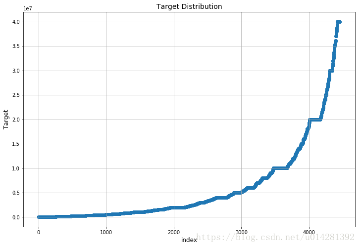

Target Histogram

plt.figure(figsize=(12,8))
plt.hist(train.target.values, bins=50)
plt.xlabel('Target', fontsize=12)
plt.title("Target Histogram", fontsize=14)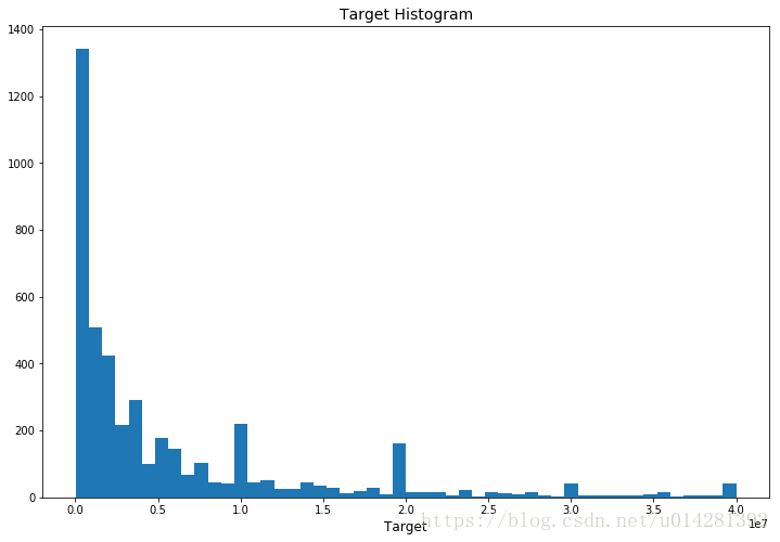

histogram (log of target)

plt.figure(figsize=(12,8))
sns.distplot( np.log1p(train.target.values), bins=50, kde=False)
plt.xlabel('Target', fontsize=12)
plt.title("Log of Target Histogram", fontsize=14)
plt.show()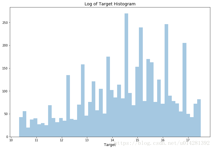

Check missing value

缺失值

# mis value count
mis_vlaue_counts = train.isnull().sum().reset_index()

# update columns name
mis_value_counts.rename(index = str,columns={'index':'Feature_name',0:'Count'},inplace=True)

(mis_value_counts.Count > 0).value_counts()

Series([], Name: Count, dtype: int64)

不存在缺失值

Check columns value type

col_type = train.dtypes.reset_index()

col_type.rename(index = str, columns={'index':'Feature_name',0:'Type'},inplace=True)

(col_type.Type).value_counts()

int64      3147
float64    1845
object        1
Name: Type, dtype: int64

object类型：１，指的是　ID

Check columns values

value_counts()

#  number of unique elements in the object
num_unique = train.nunique().reset_index()

# rename columns name
num_unique.columns = ['Col_name','Value_count']

#特征包含值的（count)
only_1_value = num_unique[num_unique.Value_count == 1]

num_unique.head()

	Col_name	Value_count
0	ID	4459
1	target	1413
2	48df886f9	32
3	0deb4b6a8	5
4	34b15f335	29

只有一个值的特征列，这些特征(256个）可以从train,test set中丢掉

only_1_value.head()

	Col_name	Value_count
28	d5308d8bc	1
35	c330f1a67	1
38	eeac16933	1
59	7df8788e8	1
70	5b91580ee	1

only_1_value.shape

(256, 2)

计算相关系数

相关系数有好几个：

• pearson
• kendall
• spearman

Pandas,Scipy,都支持相关系数的计算．

---

Scipy

from scipy.stats import spearmanr
labels = []
values = []
for col in train.columns:
    if col not in ["ID", "target"]:
        labels.append(col)
        values.append(spearmanr(train[col].values,train['target'].values)[0])
corr_df = pd.DataFrame({'col_labels':labels, 'corr_values':values})

---

Pandas贼简单,(4000+特征时间比较长）

corr_df = train.corr(method = 'spearman')['target']

Scipy : spearmanr

from tqdm import tqdm, tqdm_notebook
from scipy.stats import spearmanr
import warnings
warnings.filterwarnings('ignore')
col_names = []
cor_value = []
for col in tqdm(train.columns, ncols=100 , leave= True):
    if col not in ['ID','target']:
        col_names.append(col)
        cor_value.append(spearmanr(train[col].values, train.target.values)[0])
corrs = pd.DataFrame({'Feature_Name':col_names,'Corr_value':cor_value})
corrs = corrs.sort_values(by = 'Corr_value')

100%|██████████████████████████████████████████████████████████| 4993/4993 [00:08<00:00, 597.96it/s]

visualization corrs value

only_1_value = only_1_value.set_index('Col_name')
only_1_value.head()

	Value_count
Col_name
d5308d8bc	1
c330f1a67	1
eeac16933	1
7df8788e8	1
5b91580ee	1

corrs = corrs.set_index('Feature_Name')
corr_df = corrs.ix[list(only_1_value.index)]
# nan
corr_df.Corr_value.isnull().value_counts()

True    256
Name: Corr_value, dtype: int64

特征值只有一个的特征，跟target的相关性，为NAN

---

相关性在［-0.1~0.1]之间的特征

# 筛选出相关系数在［0.1 ~ 0.1］之间的特征
corr_df = corrs[(corrs.Corr_value > 0.1) | (corrs.Corr_value < -0.1)].reset_index()

corr_df = corr_df.set_index('Feature_Name')
corr_df.plot(kind='barh', figsize = (12,15), title='Correlation of variables')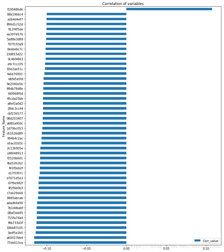

Correlation [-0.11~~0.11]

corr_df = corrs[(corrs.Corr_value > 0.11) | (corrs.Corr_value < -0.11)].reset_index()

corr_df = corr_df.set_index('Feature_Name')
corr_df.plot(kind='barh', figsize = (10,8), title='Correlation of variables')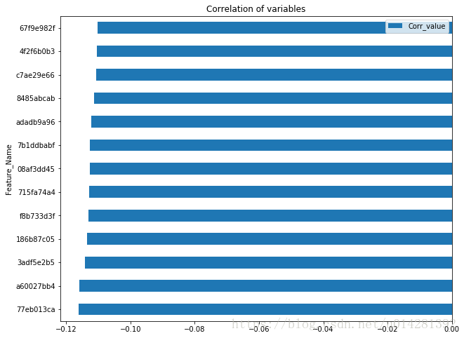

仅仅从相关性系数来看，似乎并没有相关性很强的特征．

---

利用模型来选择重要的特征

：

• ExtraTreesRegressor
• LightGBM

# num_unique == 1, columns
useless_feature_names = list(only_1_value.index)

# drop num_unique == 1的columns
train_X = train.drop(useless_feature_names + ["ID", "target"], axis=1)
test_X = test.drop(useless_feature_names + ["ID"], axis=1)
# log1p(x) = log(1+x),
train_y = np.log1p(train["target"].values)

np.log1p(x) = np.log(1+x),后面模型的结果需要执行逆操作np.expm1(x)=np.exp(x)-1

ExtraTreesRegressor(sklearn)

from sklearn import ensemble

model = ensemble.ExtraTreesRegressor(n_estimators=200, max_depth=20, max_features=0.5,
                                     n_jobs=-1, random_state=50)
model.fit(train_X, train_y)

ExtraTreesRegressor(bootstrap=False, criterion='mse', max_depth=20,
          max_features=0.5, max_leaf_nodes=None, min_impurity_decrease=0.0,
          min_impurity_split=None, min_samples_leaf=1, min_samples_split=2,
          min_weight_fraction_leaf=0.0, n_estimators=200, n_jobs=-1,
          oob_score=False, random_state=50, verbose=0, warm_start=False)

Feature Importance

# feature_importances DataFrame
feature_importances = pd.DataFrame({'Feature_name':train_X.columns,
                                    'Importances':model.feature_importances_})

# reset index
feature_importances = feature_importances.set_index('Feature_name')

# sort by importances
feature_importances = feature_importances.sort_values(by = 'Importances')

# std feature importances
std_feat_importances = np.std([tree.feature_importances_ for tree in model.estimators_],
                              axis=0)

feature_importances.iloc[-50:].plot(kind='barh',figsize = (10,20),color = 'g',
                         xerr=std_feat_importances[-50:], align='center',
                                   title='top 50 Feature Importances')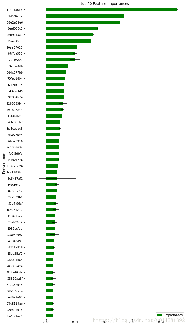

f190486d6应该是一个很重要的特征,越是重要的特征越是稳

---

Result1

$$np.expm1(x) = np.exp(x)-1$$

result = model.predict(test_X)
result = np.expm1(result)

submit = pd.DataFrame({'ID':test.ID, 'target':result})

submit.head()

	ID	target
0	000137c73	1.512680e+06
1	00021489f	1.334733e+06
2	0004d7953	2.424292e+06
3	00056a333	3.894291e+06
4	00056d8eb	1.334733e+06

Make submission file

submit.to_csv('submit3_1.csv',index = False)

测评结果

---

LightGBM

LightGBM GPU Tutorial

NVIDIA:NVS4200,加没加速没感觉，抱着试试看的态度，在老旧的Thinkpad上试了试．

def run_lgb(train_X, train_y, val_X, val_y, test_X):
    params = {
        "objective" : "regression",
        "metric" : "rmse",
        "num_leaves" : 30,
        "learning_rate" : 0.01,
        "bagging_seed" : 1884,
        "device" : "gpu",
        "gpu_platform_id" : 0,
        "gpu_device_id" : 0,
        "num_thread" : 8
    }

    train_set = lgb.Dataset(train_X, label=train_y)
    val_set = lgb.Dataset(val_X, label=val_y)

    model = lgb.train(params, train_set ,10000, valid_sets = [val_set], 
                      early_stopping_rounds = 100, verbose_eval = 200)

    result = model.predict(test_X, num_iteration = model.best_iteration)
    return result, model

采用10折交叉验证，来训练模型

kf = model_selection.KFold(n_splits = 10, shuffle = True, random_state = 1884)
pred_test_full = 0
# 10 model's Feature importances
f_imprtances = []  
for dev_index, val_index in kf.split(train_X):
    dev_X, val_X = train_X.loc[dev_index,:], train_X.loc[val_index,:]
    dev_y, val_y = train_y[dev_index], train_y[val_index]
    pred_test, model = run_lgb(dev_X, dev_y, val_X, val_y, test_X)
    # test result
    pred_test_full += pred_test/10
    # 10 model's feature importances
    f_imprtances.append(model.feature_importance())

# 结果
pred_test_full = np.expm1(pred_test_full)

Training until validation scores don't improve for 100 rounds.
[200]   valid_0's rmse: 1.42782
[400]   valid_0's rmse: 1.39864
Early stopping, best iteration is:
[437]   valid_0's rmse: 1.39731
Training until validation scores don't improve for 100 rounds.
[200]   valid_0's rmse: 1.45798
[400]   valid_0's rmse: 1.43229
Early stopping, best iteration is:
[393]   valid_0's rmse: 1.4318
Training until validation scores don't improve for 100 rounds.
[200]   valid_0's rmse: 1.46425
[400]   valid_0's rmse: 1.43454
[600]   valid_0's rmse: 1.43284
Early stopping, best iteration is:
[578]   valid_0's rmse: 1.43227
Training until validation scores don't improve for 100 rounds.
[200]   valid_0's rmse: 1.49087
[400]   valid_0's rmse: 1.47221
Early stopping, best iteration is:
[357]   valid_0's rmse: 1.47059
Training until validation scores don't improve for 100 rounds.
[200]   valid_0's rmse: 1.42226
[400]   valid_0's rmse: 1.39553
[600]   valid_0's rmse: 1.39161
Early stopping, best iteration is:
[685]   valid_0's rmse: 1.39064
Training until validation scores don't improve for 100 rounds.
[200]   valid_0's rmse: 1.46622
[400]   valid_0's rmse: 1.44762
Early stopping, best iteration is:
[461]   valid_0's rmse: 1.44708
Training until validation scores don't improve for 100 rounds.
[200]   valid_0's rmse: 1.50951
[400]   valid_0's rmse: 1.48227
[600]   valid_0's rmse: 1.47924
[800]   valid_0's rmse: 1.47827
Early stopping, best iteration is:
[702]   valid_0's rmse: 1.47819
Training until validation scores don't improve for 100 rounds.
[200]   valid_0's rmse: 1.44264
[400]   valid_0's rmse: 1.41304
Early stopping, best iteration is:
[479]   valid_0's rmse: 1.41138
Training until validation scores don't improve for 100 rounds.
[200]   valid_0's rmse: 1.46255
[400]   valid_0's rmse: 1.43719
Early stopping, best iteration is:
[450]   valid_0's rmse: 1.43618
Training until validation scores don't improve for 100 rounds.
[200]   valid_0's rmse: 1.49027
[400]   valid_0's rmse: 1.47742
Early stopping, best iteration is:
[389]   valid_0's rmse: 1.47729

RMSE ：在1.39~1.47之间，比ExtraTrees的结果要好．

# Making a submission file
submit = pd.DataFrame({'ID':test.ID, 'target':pred_test_full})

submit.to_csv('submit3_2.csv',index = False)

LightGBM在原始数据上得到的评分是1.48,这是直接在原始数据上得到的结果，这个结果可以作为baseline,在后面模型的迭代当中，其实还有很多的工作可以做，特征的选择，特征工程，数据清洗，异常值的检测等等…

---

下面是LightGBM，Feature Importances

### Feature Importance 
lgb.plot_importance(model, max_num_features=50, height=0.8, figsize=(12, 20))
plt.title("LightGBM - Feature Importance top 50", fontsize=15)

Text(0.5,1,'LightGBM - Feature Importance top 50')

---

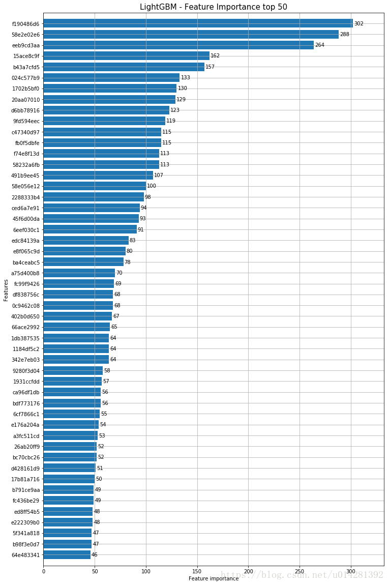
Feature Importance

Fearue_Importance = pd.DataFrame({'Feature_name':test_X.columns,
                                  'Importance':model.feature_importance()})

Fearue_Importance = Fearue_Importance.sort_values(by = 'Importance')

Fearue_Importance.to_csv('FeatureImportance_LGBM.csv',index = False)

Feature Importances & std(Feature Importance)

top50特征importance和特征importance在10个model中的std

# f_importances : 10 folds feature importances
# std_importance : every feature importance' std
std_importance = np.std(np.array(f_imprtances), axis = 0)

Fearue_Importance = Fearue_Importance.set_index('Feature_name')

Fearue_Importance.iloc[-50:].plot(kind='barh',figsize = (10,20),
                         xerr=std_importance[-50:], align='center',
                                   title='top 50 LightGBM Feature Importances')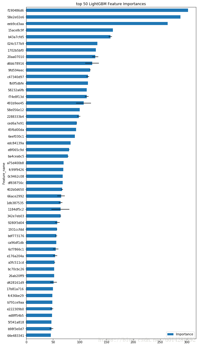

---

LightGBM & ExtraTrees,Top 300特征的交集

topx_extra_features = list(feature_importances.index)[-300:]
topx_light_features = list(Fearue_Importance.index)[-300:]

interSection = set(topx_extra_features).intersection(set(topx_light_features))

print('LightGBM & ExtraTrees Top 300 features intersection :',len(interSection))

LightGBM & ExtraTrees Top 300 features intersection : 130

Top 100

topx_extra_features = list(feature_importances.index)[-100:]
topx_light_features = list(Fearue_Importance.index)[-100:]

interSection = set(topx_extra_features).intersection(set(topx_light_features))

print('LightGBM & ExtraTrees Top 100 features intersection :',len(interSection))

LightGBM & ExtraTrees Top 100 features intersection : 56

Top 200

topx_extra_features = list(feature_importances.index)[-200:]
topx_light_features = list(Fearue_Importance.index)[-200:]

interSection = set(topx_extra_features).intersection(set(topx_light_features))

print('LightGBM & ExtraTrees Top 200 features intersection :',len(interSection))

LightGBM & ExtraTrees Top 200 features intersection : 84