Real-time Object Detection with YOLO, YOLOv2 and now YOLOv3 - YOLOv2
https://medium.com/@jonathan_hui/real-time-object-detection-with-yolo-yolov2-28b1b93e2088
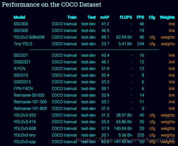
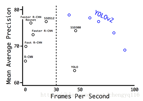
You only look once (YOLO) is an object detection system targeted for real-time processing. We will introduce YOLO, YOLOv2 and YOLO9000 in this article. For those only interested in YOLOv3, please forward to the bottom of the article. Here is the accuracy and speed comparison provided by the YOLO web site.
https://pjreddie.com/darknet/yolo/
https://medium.com/@jonathan_hui/real-time-object-detection-with-yolo-yolov2-28b1b93e2088
A demonstration from the YOLOv2.
https://www.youtube.com/watch?v=VOC3huqHrss&feature=youtu.be
YOLOv2
SSD is a strong competitor for YOLO which at one point demonstrates higher accuracy for real-time processing. Comparing with region based detectors, YOLO has higher localization errors and the recall (measure how good to locate all objects) is lower. YOLOv2 is the second version of the YOLO with the objective of improving the accuracy significantly while making it faster.
Accuracy improvements
Batch normalization
Add batch normalization in convolution layers. This removes the need for dropouts and pushes mAP up 2%.
High-resolution classifier
The YOLO training composes of 2 phases. First, we train a classifier network like VGG16. Then we replace the fully connected layers with a convolution layer and retrain it end-to-end for the object detection. YOLO trains the classifier with 224 × 224 pictures followed by 448 × 448 pictures for the object detection. YOLOv2 starts with 224 × 224 pictures for the classifier training but then retune the classifier again with 448 × 448 pictures using much fewer epochs. This makes the detector training easier and moves mAP up by 4%.
Convolutional with Anchor Boxes
As indicated in the YOLO paper, the early training is susceptible to unstable gradients. Initially, YOLO makes arbitrary guesses on the boundary boxes. These guesses may work well for some objects but badly for others resulting in steep gradient changes. In early training, predictions are fighting with each other on what shapes to specialize on.
You Only Look Once: Unified, Real-Time Object Detection
In the real-life domain, the boundary boxes are not arbitrary. Cars have very similar shapes and pedestrians have an approximate aspect ratio of 0.41.
Since we only need one guess to be right, the initial training will be more stable if we start with diverse guesses that are common for real-life objects.
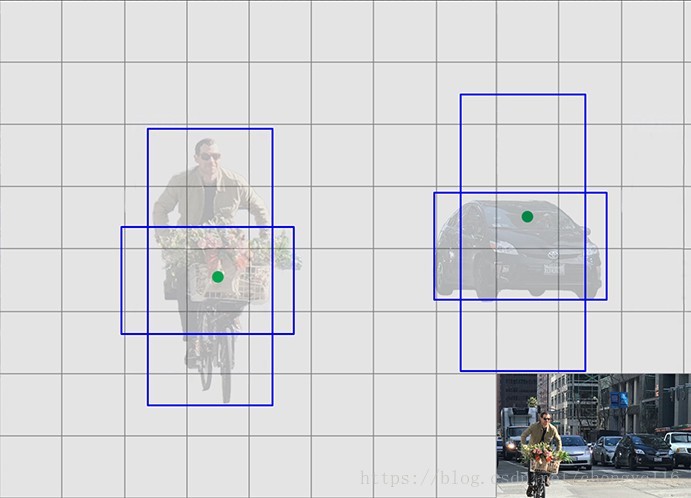
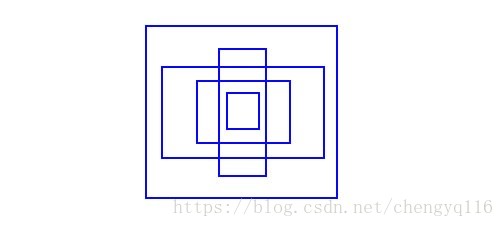
For example, we can create 5 anchor boxes with the following shapes.
Instead of predicting 5 arbitrary boundary boxes, we predict offsets to each of the anchor boxes above. If we constrain the offset values, we can maintain the diversity of the predictions and have each prediction focuses on a specific shape. So the initial training will be more stable.
In the paper, anchors are also called priors.
Here are the changes we make to the network:
Remove the fully connected layers responsible for predicting the boundary box.
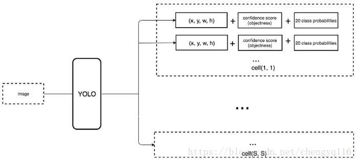
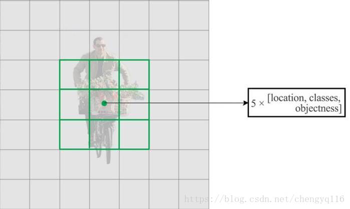
We move the class prediction from the cell level to the boundary box level. Now, each prediction includes 4 parameters for the boundary box, 1 box confidence score (objectness) and 20 class probabilities. i.e. 5 boundary boxes with 25 parameters: 125 parameters per grid cell. Same as YOLO, the objectness prediction still predicts the IOU of the ground truth and the proposed box.
To generate predictions with a shape of 7 × 7 × 125, we replace the last convolution layer with three 3 × 3 convolutional layers each outputting 1024 output channels. Then we apply a final 1 × 1 convolutional layer to convert the 7 × 7 × 1024 output into 7 × 7 × 125. (See the section on DarkNet for the details.)
Change the input image size from 448 × 448 to 416 × 416. This creates an odd number spatial dimension (7 × 7 v.s. 8 × 8 grid cell). The center of a picture is often occupied by a large object. With an odd number grid cell, it is more certain on where the object belongs.
Just we have a tendency to center objects in taking pictures or in some case, we just follow behind a car. So if your dataset has more centered object that trick will improve your mAP.

Remove one pooling layer to make the spatial output of the network to 13 × 13 (instead of 7 × 7).
Anchor boxes decrease mAP slightly from 69.5 to 69.2 but the recall improves from 81% to 88%. i.e. even the accuracy is slightly decreased but it increases the chances of detecting all the ground truth objects.
Dimension Clusters
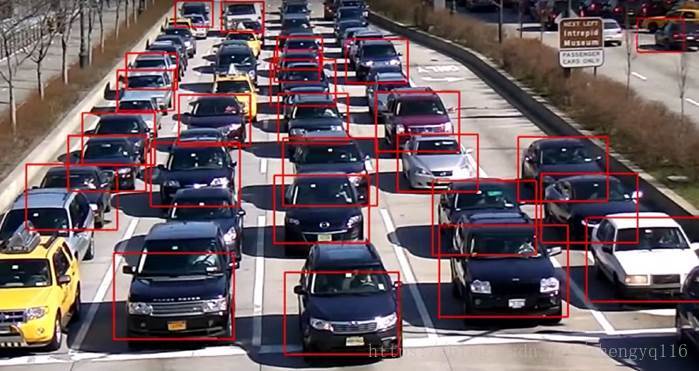
In many problem domains, the boundary boxes have strong patterns. For example, in the autonomous driving, the 2 most common boundary boxes will be cars and pedestrians at different distances. To identify the top-K boundary boxes that have the best coverage for the training data, we run K-means clustering on the training data to locate the centroids of the top-K clusters.
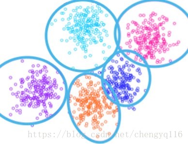
https://mapr.com/blog/monitoring-real-time-uber-data-using-spark-machine-learning-streaming-and-kafka-api-part-1/
Since we are dealing with boundary boxes rather than points, we cannot use the regular spatial distance to measure datapoint distances. No surprise, we use IoU.
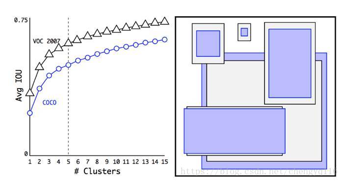
On the left, we plot the average IoU between the anchors and the ground truth boxes using different numbers of clusters (anchors). As the number of anchors increases, the accuracy improvement plateaus. For the best return, YOLO settles down with 5 anchors. On the right, it displays the 5 anchors’ shapes. The purplish-blue rectangles are selected from the COCO dataset while the black border rectangles are selected from the VOC2007. In both cases, we have more thin and tall anchors indicating that real-life boundary boxes are not arbitrary.
Unless we are comparing YOLO and YOLOv2, we will reference YOLOv2 as YOLO for now.
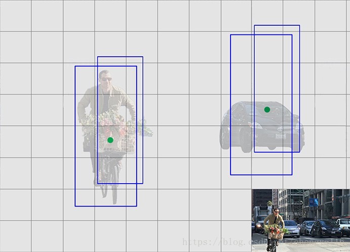
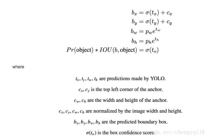
Direct location prediction
We make predictions on the offsets to the anchors. Nevertheless, if it is unconstrained, our guesses will be randomized again. YOLO predicts 5 parameters (tx, ty, tw, th, and to) and applies the sigma function to constraint its possible offset range.
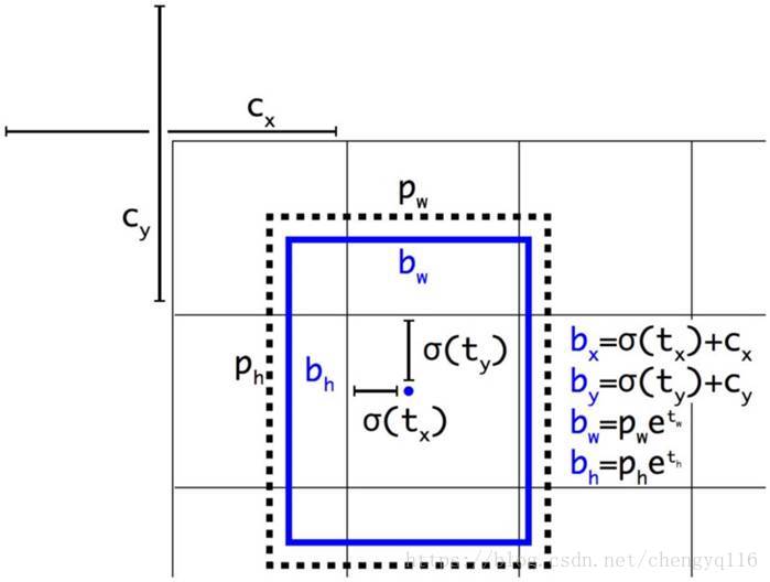
Here is the visualization. The blue box below is the predicted boundary box and the dotted rectangle is the anchor.
YOLO9000: Better, Faster, Stronger
With the use of k-means clustering (dimension clusters) and the improvement mentioned in this section, mAP increases 5%.
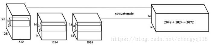
Fine-Grained Features
细粒度特征
Convolution layers decrease the spatial dimension gradually. As the corresponding resolution decreases, it is harder to detect small objects. Other object detectors like SSD locate objects from different layers of feature maps. So each layer specializes at a different scale. YOLO adopts a different approach called passthrough. It reshapes the 28 × 28 × 512 layer to 14 × 14 × 2048. Then it concatenates with the original 14 × 14 ×1024 output layer. Now we apply convolution filters on the new 14 × 14 × 3072 layer to make predictions.
Multi-Scale Training
After removing the fully connected layers, YOLO can take images of different sizes. If the width and height are doubled, we are just making 4x output grid cells and therefore 4x predictions. Since the YOLO network downsamples the input by 32, we just need to make sure the width and height is a multiple of 32. During training, YOLO takes images of size 320×320, 352×352, … and 608×608 (with a step of 32). For every 10 batches, YOLOv2 randomly selects another image size to train the model. This acts as data augmentation and forces the network to predict well for different input image dimension and scale. In additional, we can use lower resolution images for object detection at the cost of accuracy. This can be a good tradeoff for speed on low GPU power devices. At 288 × 288 YOLO runs at more than 90 FPS with mAP almost as good as Fast R-CNN. At high-resolution YOLO achieves 78.6 mAP on VOC 2007.
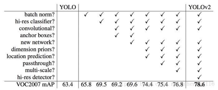
Accuracy
Here is the accuracy improvements after applying the techniques discussed so far:
Accuracy comparison for different detectors:
Speed improvement
GoogLeNet
VGG16 requires 30.69 billion floating point operations for a single pass over a 224 × 224 image versus 8.52 billion operations for a customized GoogLeNet. We can replace the VGG16 with the customized GoogLeNet. However, YOLO pays a price on the top-5 accuracy for ImageNet: accuracy drops from 90.0% to 88.0%.
DarkNet
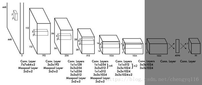
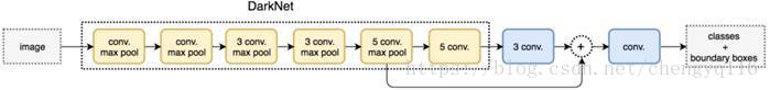
We can further simplify the backbone CNN used. Darknet requires 5.58 billion operations only. With DarkNet, YOLO achieves 72.9% top-1 accuracy and 91.2% top-5 accuracy on ImageNet. Darknet uses mostly 3 × 3 filters to extract features and 1 × 1 filters to reduce output channels. It also uses global average pooling to make predictions. Here is the detail network description:
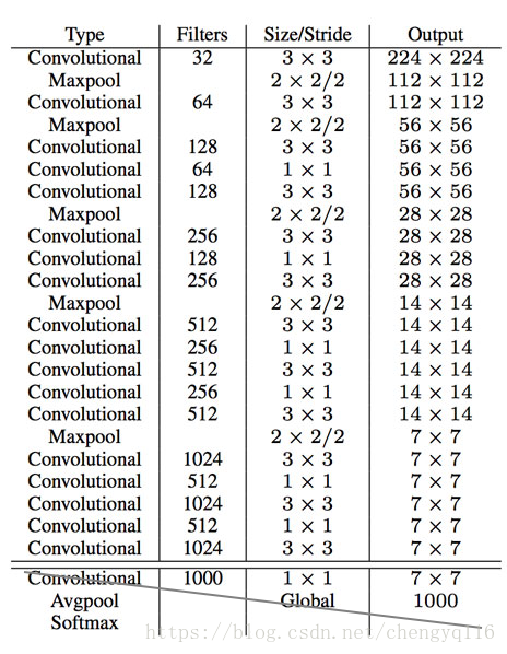
We replace the last convolution layer (the cross-out section) with three 3 × 3 convolutional layers each outputting 1024 output channels. Then we apply a final 1 × 1 convolutional layer to convert the 7 × 7 × 1024 output into 7 × 7 × 125. (5 boundary boxes each with 4 parameters for the box, 1 objectness score and 20 conditional class probabilities)
Training
YOLO is trained with the ImageNet 1000 class classification dataset in 160 epochs: using stochastic gradient descent with a starting learning rate of 0.1, polynomial rate decay with a power of 4, weight decay of 0.0005 and momentum of 0.9. In the initial training, YOLO uses 224 × 224 images, and then retune it with 448 × 448 images for 10 epochs at a 10-3 learning rate. After the training, the classifier achieves a top-1 accuracy of 76.5% and a top-5 accuracy of 93.3%.
Then the fully connected layers and the last convolution layer is removed for a detector. YOLO adds three 3 × 3 convolutional layers with 1024 filters each followed by a final 1 × 1 convolutional layer with 125 output channels. (5 box predictions each with 25 parameters) YOLO also add a passthrough layer. YOLO trains the network for 160 epochs with a starting learning rate of 10-3, dividing it by 10 at 60 and 90 epochs. YOLO uses a weight decay of 0.0005 and momentum of 0.9.
Classification
Datasets for object detection have far fewer class categories than those for classification. To expand the classes that YOLO can detect, YOLO proposes a method to mix images from both detection and classification datasets during training. It trains the end-to-end network with the object detection samples while backpropagates the classification loss from the classification samples to train the classifier path.
This approach encounters a few challenges:
- How do we merge class labels from different datasets? In particular, object detection datasets and different classification datasets uses different labels.
- Any merged labels may not be mutually exclusive, for example, Norfolk terrier in ImageNet and dog in COCO. Since it is not mutually exclusive, we can not use softmax to compute the probability.
Hierarchical classification
层次分类
Without going into details, YOLO combines labels in different datasets to form a tree-like structure WordTree. The children form an is-a relationship with its parent like biplane is a plane. But the merged labels are now not mutually exclusive.
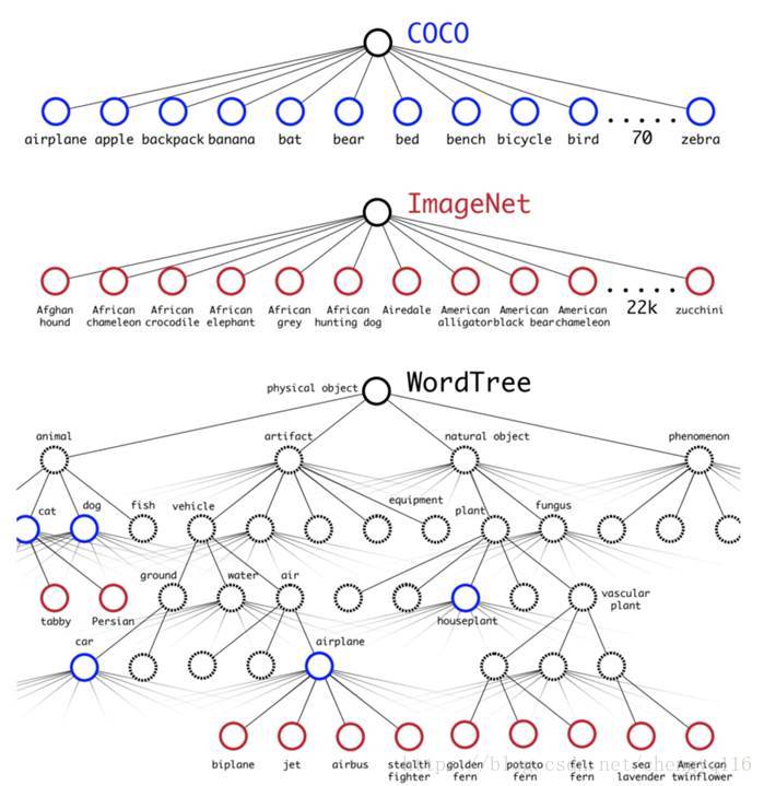
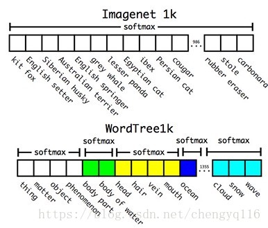
Let’s simplify the discussion using the 1000 class ImageNet. Instead of predicting 1000 labels in a flat structure, we create the corresponding WordTree which has 1000 leave nodes for the original labels and 369 nodes for their parent classes. Originally, YOLO predicts the class score for the biplane. But with the WordTree, it now predicts the score for the biplane given it is an airplane.

Since

we can apply a softmax function to compute the probability

from the scores of its own and the siblings. The difference is, instead of one softmax operations, YOLO performs multiple softmax operations for each parent’s children.
The class probability is then computed from the YOLO predictions by going up the WordTree.
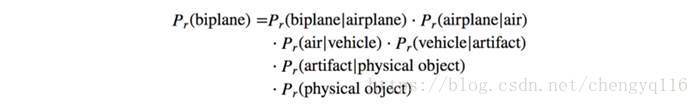
For classification, we assume an object is already detected and therefore Pr(physical object)=1.
One benefit of the hierarchy classification is that when YOLO cannot distinguish the type of airplane, it gives a high score to the airplane instead of forcing it into one of the sub-categories.
When YOLO sees a classification image, it only backpropagates classification loss to train the classifier. YOLO finds the bounding box that predicts the highest probability for that class and it computes the classification loss as well as those from the parents. (If an object is labeled as a biplane, it is also considered to be labeled as airplane, air, vehicle… ) This encourages the model to extract features common to them. So even we have never trained a specific class of objects for object detection, we can still make such predictions by generalizing predictions from related objects.
In object detection, we set Pr(physical object) equals to the box confidence score which measures whether the box has an object. YOLO traverses down the tree, taking the highest confidence path at every split until it reaches some threshold and YOLO predicts that object class.
YOLO9000
YOLO9000 extends YOLO to detect objects over 9000 classes using hierarchical classification with a 9418 node WordTree. It combines samples from COCO and the top 9000 classes from the ImageNet. YOLO samples four ImageNet data for every COCO data. It learns to find objects using the detection data in COCO and to classify these objects with ImageNet samples.
During the evaluation, YOLO test images on categories that it knows how to classify but not trained directly to locate them, i.e. categories that do not exist in COCO. YOLO9000 evaluates its result from the ImageNet object detection dataset which has 200 categories. It shares about 44 categories with COCO. Therefore, the dataset contains 156 categories that have never been trained directly on how to locate them. YOLO extracts similar features for related object types. Hence, we can detect those 156 categories by simply from the feature values.
YOLO9000 gets 19.7 mAP overall with 16.0 mAP on those 156 categories. YOLO9000 performs well with new species of animals not found in COCO because their shapes can be generalized easily from their parent classes. However, COCO does not have bounding box labels for any type of clothing so the test struggles with categories like “sunglasses”.
Wordbook
grid cell:网格单元
Santa Claus [ˈsæntə klɔ:z]:圣诞老人
linear regression:线性回归
square root:平方根,二次根
diverse [daɪ’vɜːs; ‘daɪvɜːs]:adj. 不同的,多种多样的,变化多的
aspect ratio:纵横比,屏幕高宽比
An autonomous car (also known as a driverless car and a self-driving car) is a vehicle that is capable of sensing its environment and navigating without human input.
plateau [‘plætəʊ]:n. 高原,稳定水平,托盘,平顶女帽 vi. 达到平衡,达到稳定时期
purplish blue:紫蓝,海军蓝,藏蓝
Visual Object Classes,VOC:视觉目标分类
Pattern Analysis, Statistical Modelling and Computational Learning,PASCAL
fine-grained:adj. 细粒的,有细密纹理的 adj. 详细的,深入的
concatenate [kən’kætɪneɪt]:vt. 连结,使连锁 adj. 连结的,连锁的
high-resolution,hi-res:高分辨率
cross out:删去,注销
epoch [‘iːpɒk; ‘epɒk]:n. 世,新纪元,新时代,时间上的一点
mutually exclusive:互相排斥的
Norfolk Terrier:诺福克梗 (犬种名)
sunglass [’sʌnɡlæs]:n. 太阳眼镜,聚集日光引火的凸透镜
biplane [‘baɪpleɪn]:n. 复翼飞机,双翼飞机
backpropagation:n. 反向传播
References
https://medium.com/@jonathan_hui/real-time-object-detection-with-yolo-yolov2-28b1b93e2088