加州房价预测项目精细解释

此处选择StatLib的加州房产价格数据集，该数据集是基于1990年加州普查的数据

一、项目概览

利用加州普查数据，建立一个加州房价模型，这个数据包含每个街区组的人口、收入的中位数、房价中位数等指标。街区组是美国调查局发布样本数据的最小地理单位（600到3000人），简称“街区”。

目标：模型利用该数据进行学习，然后根据其他指标，预测任何街区的房价中位数

二、划定问题

1、应该认识到，该问题的商业目标是什么？

建立模型不可能是最终目标，而是公司的受益情况，这决定了如何划分问题，选择什么算法，评估模型的指标和微调等等

你建立的模型的输出（一个区的房价中位数）会传递给另一个机器学习系统，也有其他信号传入该系统，从而确定该地区是否值得投资。

2、第二个问题是现在的解决方案效果如何？

比如现在截取的房价是靠专家手工估计的，专家队伍收集最新的关于一个区的信息（不包括房价的中位数），他们使用复杂的规则进行估计，这种方法浪费资源和时间，而且效果不理想，误差率大概有15%。

开始设计系统

1、划定问题：监督与否、强化学习与否、分类与否、批量学习或线上学习

2、确定问题：

• 该问题是一个典型的监督学习任务，我们使用的是有标签的训练样本，每个实例都有预定的产出，即街区的房价中位数

• 并且是一个典型的回归任务，因为我们要预测的是一个值。

  更细致一些：该问题是一个多变量的回归问题，因为系统要使用多个变量来预测结果

• 最后，没有连续的数据流进入系统，没有特别需求需要对数据变动来做出快速适应，数据量不大可以放到内存中，因此批量学习就够了

  提示：如果数据量很大，你可以要么在多个服务器上对批量学习做拆分（使用Mapreduce技术），或是使用线上学习

三、选择性能指标

回归问题的典型指标是均方根误差（RMSE），均方根误差测量的是系统预测误差的标准差，例如RMSE=50000，意味着68%的系统预测值位于实际值的50000美元误差
以内，95%的预测值位于实际值的100000美元以内，一个特征通常都符合高斯分布，即满足68-95-99.7规则，大约68%的值位于1$\sigma$内，95%的值位于$2 \sigma$内，99.7%的值位于$3\sigma$内，此处的$\sigma=50000$，RMSE计算如下：

$$RMSE(X,h)=\sqrt{\frac{1}{m}\sum_{i=1}^m(h(X^i)-y^{(i)})^2}$$

虽然大多数时候的RMSE是回归任务可靠的性能指标，在有些情况下，你可能需要另外的函数，例如，假设存在许多异常的街区，此时可能需要使用平均绝对误差（MAE）,也称为曼哈顿范数，因为其测量了城市中的两点，沿着矩形的边行走的距离：

$$MAE(X,h)=\frac{1}{m}\sum_{i=1}^m|h(X^i)-y^{(i)}|$$

范数的指数越高，就越关注大的值而忽略小的值，这就是为什么RMSE比MAE对异常值更敏感的原因，但是当异常值是指数分布的时候（类似正态曲线），RMSE就会表现的很好

四、核实假设

最好列出并核对迄今做出的假设，这样可以尽早发现严重的问题，例如，系统输出的街区房价会传入到下游的机器学习系统，我们假设这些价格确实会被当做街区房价使用，但是如果下游系统将价格转化为分类（便宜、昂贵、中等等），然后使用这些分类来进行判定的话，就将回归问题变为分类问题，能否获得准确的价格已经不是很重要了。

此时将回归问题变成了分类问题

五、获取数据

下面是获取数据的函数：

import os
import tarfile
from six.moves import urllib

DOWNLOAD_ROOT="https://raw.githubusercontent.com/ageron/handson-ml/master/"
HOUSING_PATH="datasets/housing"
HOUSING_URL=DOWNLOAD_ROOT+HOUSING_PATH+"housing.tgz"

def fetch_housing_data(housing_url=HOUSING_URL,housing_path=HOUSING_PATH):
     # os.path.isdir():判断某一路径是否为目录
     # os.makedirs():  递归创建目录
    if not os.path.isdir(housing_path):
        os.makedirs(housing_path)
     # 获取当前目录，并组合成新目录
    tgz_path=os.path.join(housing_path,"housing.tgz") 
     # 将url表示的对象复制到本地文件，
    urllib.request.urlretrieve(housing_url,tgz_path)
    housing_tgz=trafile.open(tgz_path)
    housing_tgz.extractall(path=housing_path)
    housing_tgz.close()

调用fetch_housing_data()的时候，就会在工作空间创建一个datasets/housing目录，下载housing.tgz文件，并解压出housing.csv 然后使用pandas加载数据：

import pandas as pd

def load_housing_data(housing_path=HOUSING_PATH):
    csv_path=os.path.join(housing_path,"housing.csv")
    return pd.read_csv(csv_path)
    # csv文件是用逗号分开的一列列数据文件

该函数会返回一个包含所有数据的pandas的DataFrame对象，DataFrame对象是表格型的数据结构，提供有序的列和不同类型的列值

查看数据结构

1、使用head()方法查看前五行

housing=load_housing_data()
housing.head()

.dataframe thead tr:only-child th { text-align: right; } .dataframe thead th { text-align: left; } .dataframe tbody tr th { vertical-align: top; }

	longitude	latitude	housing_median_age	total_rooms	total_bedrooms	population	households	median_income	median_house_value	ocean_proximity
0	-122.23	37.88	41.0	880.0	129.0	322.0	126.0	8.3252	452600.0	NEAR BAY
1	-122.22	37.86	21.0	7099.0	1106.0	2401.0	1138.0	8.3014	358500.0	NEAR BAY
2	-122.24	37.85	52.0	1467.0	190.0	496.0	177.0	7.2574	352100.0	NEAR BAY
3	-122.25	37.85	52.0	1274.0	235.0	558.0	219.0	5.6431	341300.0	NEAR BAY
4	-122.25	37.85	52.0	1627.0	280.0	565.0	259.0	3.8462	342200.0	NEAR BAY

每一行表示一个街区，共有10个属性，经度、纬度、房屋年龄中位数、总房间数、总卧室数、人口数、家庭数、收入中位数、房屋价值中位数、离大海的距离

2、使用info()方法可以快速查看数据的描述，特别是总行数、每个属性的类型和非空值的数量

housing.info()

housing["ocean_proximity"].value_counts()

housing.describe()

.dataframe thead tr:only-child th { text-align: right; } .dataframe thead th { text-align: left; } .dataframe tbody tr th { vertical-align: top; }

	longitude	latitude	housing_median_age	total_rooms	total_bedrooms	population	households	median_income	median_house_value
count	20640.000000	20640.000000	20640.000000	20640.000000	20433.000000	20640.000000	20640.000000	20640.000000	20640.000000
mean	-119.569704	35.631861	28.639486	2635.763081	537.870553	1425.476744	499.539680	3.870671	206855.816909
std	2.003532	2.135952	12.585558	2181.615252	421.385070	1132.462122	382.329753	1.899822	115395.615874
min	-124.350000	32.540000	1.000000	2.000000	1.000000	3.000000	1.000000	0.499900	14999.000000
25%	-121.800000	33.930000	18.000000	1447.750000	296.000000	787.000000	280.000000	2.563400	119600.000000
50%	-118.490000	34.260000	29.000000	2127.000000	435.000000	1166.000000	409.000000	3.534800	179700.000000
75%	-118.010000	37.710000	37.000000	3148.000000	647.000000	1725.000000	605.000000	4.743250	264725.000000
max	-114.310000	41.950000	52.000000	39320.000000	6445.000000	35682.000000	6082.000000	15.000100	500001.000000

卧室总数total_bedrooms为20433，所以空值被忽略了，std是标准差，揭示数值的分散度，25%的街区房屋年龄中位数小于18，50%的小于19，75%的小于37，这些值通常称为第25个百分位数（第一个四分位数）、中位数、第75个百分位数（第三个四分位数），不同大小的分位数如果很接近，说明数据很集中，集中在某个段里。

5、另外一种快速了解数据类型的方法是画出每个数值属性的柱状图housing.hist()

import matplotlib.pyplot as plt
housing.hist(bins=50,figsize=(20,15))
plt.show()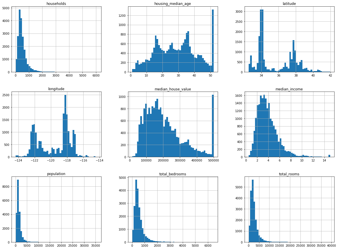

① 收入中位不是美元，而是经过缩放调整的，过高收入的中位数会变为15，过低会变成0.5，也就是设置了阈值。

② 房屋年龄中位数housing_median_age和房屋价值中位数median_house_value也被设了上限，房屋价值中位数是目标属性，我们的机器学习算法学习到的价格不会超过该界限。有两种处理方法：

• 对于设了上限的标签，重新收集合适的标签
• 将这些街区从训练集中移除，也从测试集中移除，因为这会导致不准确

③ 这些属性有不同的量度，会在后续讨论特征缩放

④ 柱状图多为长尾的，是有偏的，对于某些机器学习算法，这会使得检测规律变得困难，后面我们将尝试变换处理这些属性，使其成为正态分布，比如log变换。

六、创建测试集

测试集在这个阶段就要进行分割，因为如果查看了测试集，就会不经意的按照测试集中的规律来选择某个特定的机器学习模型，当再使用测试集进行误差评估的时候，就会发生过拟合，在实际系统中表现很差。

随机挑选一些实例，一般是数据集的20%

from sklearn.model_selection import train_test_split
train_set,test_set=train_test_split(housing,test_size=0.2,random_state=42)
test_set.head()

.dataframe thead tr:only-child th { text-align: right; } .dataframe thead th { text-align: left; } .dataframe tbody tr th { vertical-align: top; }

	longitude	latitude	housing_median_age	total_rooms	total_bedrooms	population	households	median_income	median_house_value	ocean_proximity
20046	-119.01	36.06	25.0	1505.0	NaN	1392.0	359.0	1.6812	47700.0	INLAND
3024	-119.46	35.14	30.0	2943.0	NaN	1565.0	584.0	2.5313	45800.0	INLAND
15663	-122.44	37.80	52.0	3830.0	NaN	1310.0	963.0	3.4801	500001.0	NEAR BAY
20484	-118.72	34.28	17.0	3051.0	NaN	1705.0	495.0	5.7376	218600.0	<1H OCEAN
9814	-121.93	36.62	34.0	2351.0	NaN	1063.0	428.0	3.7250	278000.0	NEAR OCEAN

上述为随机的取样方法，当数据集很大的时候，尤其是和属性数量相比很大的时候，通常是可行的，但是如果数据集不大，就会有采样偏差的风险，当一个调查公司想要对1000个人进行调查，不能是随机取1000个人，而是要保证有代表性，美国人口的51.3%是女性，48.7%是男性，所以严谨的调查需要保证样本也是这样的比例：513名女性，487名男性，这称为分层采样。

分层采样：将人群分成均匀的子分组，称为分层，从每个分层去取合适数量的实例，保证测试集对总人数具有代表性

如果随机采样的话，会产生严重的偏差。

若我们已知收入的中位数对最终结果的预测很重要，则我们要保证测试集可以代表整体数据集中的多种收入分类，因为收入中位数是一个连续的数值属性，首先需要创建一个收入类别属性，再仔细看一下收入中位数的柱状图

housing["median_income"].hist()
plt.show()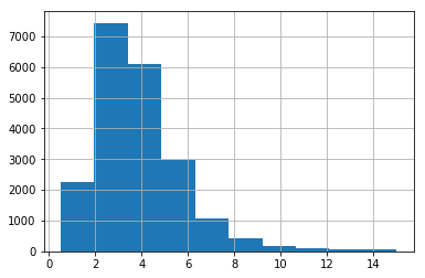

大多数的收入的中位数都在2-5（万美元），但是一些收入中位数会超过6，数据集中的每个分层都要有足够的实例位于你的数据中，这点很重要，否则，对分层重要性的评估就会有偏差，这意味着不能有过多的分层，并且每个分层都要足够大。

随机切分的方式不是很合理，因为随机切分会将原本的数据分布破坏掉，比如收入、性别等，可以采用分桶、等频切分等方式，保证每个桶内的数量和原本的分布接近，来完成切分，保证特性分布是很重要的。

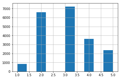
创建收入的类别属性：利用中位数/1.5,ceil()对值进行舍入，以产生离散的分类，然后将所有大于5的分类归类于分类5

# Divide by 1.5 to limit the number of income categories
import numpy as np
housing["income_cat"]=np.ceil(housing["median_income"]/1.5)
housing["income_cat"].head()

0 6.0 1 6.0 2 5.0 3 4.0 4 3.0 Name: income_cat, dtype: float64

# Label those above 5 as 5
housing["income_cat"].where(housing["income_cat"]<5,5.0,inplace=True)

housing["income_cat"].hist()
plt.show()

 根据收入分类，进行分层采样，使用sklearn的stratifiedShuffleSplit类

from sklearn.model_selection import StratifiedShuffleSplit
split=StratifiedShuffleSplit(n_splits=1,test_size=0.2,random_state=42)

for train_index,test_index in split.split(housing,housing["income_cat"]):
    strat_train_set=housing.loc[train_index]
    strat_test_set=housing.loc[test_index]

查看分层抽样之后测试集的分布状况

strat_test_set["income_cat"].value_counts()/len(strat_test_set)

3.0 0.350533 2.0 0.318798 4.0 0.176357 5.0 0.114583 1.0 0.039729 Name: income_cat, dtype: float64

len(strat_test_set)

4128 查看原始数据集的分布状况

housing["income_cat"].value_counts()/len(housing)
# .value_counts():确认数据出现的频数

3.0 0.350581 2.0 0.318847 4.0 0.176308 5.0 0.114438 1.0 0.039826 Name: income_cat, dtype: float64

len(housing)

20640

可以看出，测试集和原始数据集的分布状况几乎一致

对分层采样和随机采样的对比：

def income_cat_proportions(data):
    return data["income_cat"].value_counts()/len(data)

train_set,test_set=train_test_split(housing,test_size=0.2,random_state=42)
compare_props=pd.DataFrame({"Overall":income_cat_proportions(housing),
                           "Stratified":income_cat_proportions(strat_test_set),
                           "Random":income_cat_proportions(test_set),}).sort_index()
compare_props["Rand. %error"]=100*compare_props["Random"]/compare_props["Overall"]-100
compare_props["Strat. %error"]=100*compare_props["Random"]/compare_props["Overall"]-100
compare_props

.dataframe thead tr:only-child th { text-align: right; } .dataframe thead th { text-align: left; } .dataframe tbody tr th { vertical-align: top; }

	Overall	Random	Stratified	Rand. %error	Strat. %error
1.0	0.039826	0.040213	0.039729	0.973236	0.973236
2.0	0.318847	0.324370	0.318798	1.732260	1.732260
3.0	0.350581	0.358527	0.350533	2.266446	2.266446
4.0	0.176308	0.167393	0.176357	-5.056334	-5.056334
5.0	0.114438	0.109496	0.114583	-4.318374	-4.318374

上述表格对比了总数据集、分层采样测试集、纯随机采样测试集的收入分类比例，可以看出分层采样测试集的收入分类比例与总数据集几乎相同，而随机采样数据集偏差严重

housing.head(20)

.dataframe thead tr:only-child th { text-align: right; } .dataframe thead th { text-align: left; } .dataframe tbody tr th { vertical-align: top; }

	longitude	latitude	housing_median_age	total_rooms	total_bedrooms	population	households	median_income	median_house_value	ocean_proximity	income_cat
0	-122.23	37.88	41.0	880.0	129.0	322.0	126.0	8.3252	452600.0	NEAR BAY	5.0
1	-122.22	37.86	21.0	7099.0	1106.0	2401.0	1138.0	8.3014	358500.0	NEAR BAY	5.0
2	-122.24	37.85	52.0	1467.0	190.0	496.0	177.0	7.2574	352100.0	NEAR BAY	5.0
3	-122.25	37.85	52.0	1274.0	235.0	558.0	219.0	5.6431	341300.0	NEAR BAY	4.0
4	-122.25	37.85	52.0	1627.0	280.0	565.0	259.0	3.8462	342200.0	NEAR BAY	3.0
5	-122.25	37.85	52.0	919.0	213.0	413.0	193.0	4.0368	269700.0	NEAR BAY	3.0
6	-122.25	37.84	52.0	2535.0	489.0	1094.0	514.0	3.6591	299200.0	NEAR BAY	3.0
7	-122.25	37.84	52.0	3104.0	687.0	1157.0	647.0	3.1200	241400.0	NEAR BAY	3.0
8	-122.26	37.84	42.0	2555.0	665.0	1206.0	595.0	2.0804	226700.0	NEAR BAY	2.0
9	-122.25	37.84	52.0	3549.0	707.0	1551.0	714.0	3.6912	261100.0	NEAR BAY	3.0
10	-122.26	37.85	52.0	2202.0	434.0	910.0	402.0	3.2031	281500.0	NEAR BAY	3.0
11	-122.26	37.85	52.0	3503.0	752.0	1504.0	734.0	3.2705	241800.0	NEAR BAY	3.0
12	-122.26	37.85	52.0	2491.0	474.0	1098.0	468.0	3.0750	213500.0	NEAR BAY	3.0
13	-122.26	37.84	52.0	696.0	191.0	345.0	174.0	2.6736	191300.0	NEAR BAY	2.0
14	-122.26	37.85	52.0	2643.0	626.0	1212.0	620.0	1.9167	159200.0	NEAR BAY	2.0
15	-122.26	37.85	50.0	1120.0	283.0	697.0	264.0	2.1250	140000.0	NEAR BAY	2.0
16	-122.27	37.85	52.0	1966.0	347.0	793.0	331.0	2.7750	152500.0	NEAR BAY	2.0
17	-122.27	37.85	52.0	1228.0	293.0	648.0	303.0	2.1202	155500.0	NEAR BAY	2.0
18	-122.26	37.84	50.0	2239.0	455.0	990.0	419.0	1.9911	158700.0	NEAR BAY	2.0
19	-122.27	37.84	52.0	1503.0	298.0	690.0	275.0	2.6033	162900.0	NEAR BAY	2.0

现在需要删除income_cat属性，使数据回到最初的状态,利用.drop()来删除某一行/列

for set_ in (strat_train_set,strat_test_set):
    set_.drop("income_cat",axis=1,inplace=True)

我们通过大量时间来生成测试集的原因是：测试集通常被忽略，但实际上是机器学习非常重要的一部分，还有，生成测试集过程中有很多思路对后面的交叉验证讨论是非常有帮助的。

七、数据探索和可视化、发现规律

目前只是查看了数据，现在需要对数据有整体的了解，更深入的探索数据，现在只研究训练集，可以创建一个副本，以免损伤训练集。

housing=strat_train_set.copy()

1、地理数据可视化

housing.plot(kind="scatter",x="longitude",y="latitude")
plt.show()

 上图看起来很像加州，但是看不出有什么特别地规律，将alpha设为0.1，就可以看出数据点的密度

housing.plot(kind="scatter",x="longitude",y="latitude",alpha=0.1)
plt.show()
# 颜色越深，表示叠加越多

 上图可以非常清楚的看到高密度区域，弯区、洛杉矶和圣迭戈，以及中央谷。

2、房价可视化

housing.plot(kind="scatter",x="longitude",y="latitude",alpha=0.4,
             s=housing["population"]/100,label="population",
             c="median_house_value",cmap=plt.get_cmap("jet"),colorbar=True,sharex=False)

plt.legend()
plt.show()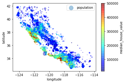

每个圈的半径表示街区的人口（s），颜色代表价格（c），我们用预先定义的名为jet的颜色图（cmap），其范围从蓝色（低价）到红色（高价）

上图说明房价和位置（比如离海的距离）和人口密度联系密切，可以使用聚类的算法来检测主要的聚集，用一个新的特征值测量聚集中心的距离，

八、查找关联

1、person系数：

因为数据集并不是很大，所以可以使用corr()的方法来计算出每对属性间的标准相关系数，也称为person相关系数

corr_matrix=housing.corr()

查看每个属性和房价中位数的关联度

corr_matrix["median_house_value"].sort_values(ascending=False)

median_house_value 1.000000 median_income 0.687160 total_rooms 0.135097 housing_median_age 0.114110 households 0.064506 total_bedrooms 0.047689 population -0.026920 longitude -0.047432 latitude -0.142724 Name: median_house_value, dtype: float64 相关系数的范围是-1~1，接近1的时候强正相关，接近-1的时候，强负相关，接近于0的时候，意味着没有线性相关性。 相关系数只策略线性关系，可能完全忽略非线性关系，下图的最后一行就是非线性关系的例子

from IPython.display import Image
Image(filename='E:/person.png')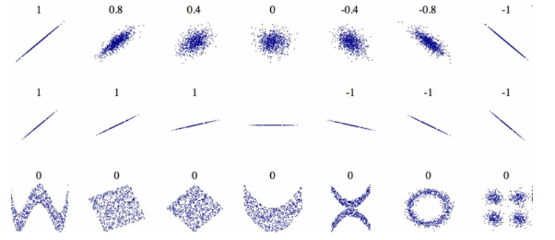

2、scatter_matrix()函数：

可以绘制每个数值属性对每个其他数值属性的图，因为现在有11个数值属性，可以得到$11^2=121$张图，所以只关注几个和房价中位数最有可能相关的属性。

from pandas.tools.plotting import scatter_matrix

attributes=["median_house_value","median_income","total_rooms","housing_median_age"]
scatter_matrix(housing[attributes],figsize=(12,8))
plt.show()

C:\Anaconda\lib\site-packages\ipykernel\__main__.py:4: FutureWarning: 'pandas.tools.plotting.scatter_matrix' is deprecated, import 'pandas.plotting.scatter_matrix' instead.

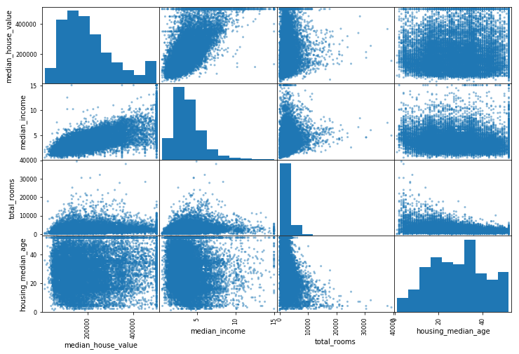
如果pandas将每个变量对自己作图，主对角线（左上到右下）都会是直线，所以pandas展示的是每个属性的柱状图

最有希望用来预测房价中位数的属性是收入中位数，因此将这张图放大：

housing.plot(kind="scatter",x="median_income",y="median_house_value",alpha=0.1)
plt.show()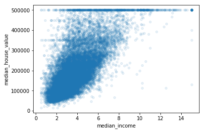

该图说明了几点：

• 首先，相关性非常高，可以清晰的看到向上的趋势，并且数据点不是很分散
• 其次，图中在280000美元、350000美元、450000美元、500000美元都出现了水平线，可以去除对应的街区，防止过拟合

九、属性组合实验

给算法准备数据之前，需要做的最后一件事是尝试多种属性组合，例如，你不知道某个街区有多少户，该街区的总房间数就没有什么用，你真正需要的是每户有几个房间，同样的，总卧室数也不重要，你可能需要将其与房间数进行比较，每户的人口数也是一个有趣的组合，可以创建这些新属性。

housing["roomes_per_household"]=housing["total_rooms"]/housing["households"]
housing["bedrooms_per_rooms"]=housing["total_bedrooms"]/housing["total_rooms"]
housing["population_per_household"]=housing["population"]/housing["households"]
corr_matrix=housing.corr()
corr_matrix["median_house_value"].sort_values(ascending=False)# False:降序

median_house_value 1.000000 median_income 0.687160 roomes_per_household 0.146285 total_rooms 0.135097 housing_median_age 0.114110 households 0.064506 total_bedrooms 0.047689 population_per_household -0.021985 population -0.026920 longitude -0.047432 latitude -0.142724 bedrooms_per_rooms -0.259984 Name: median_house_value, dtype: float64 与总房间数/卧室数相比，新的特征“每个房子中的卧室数 bedrooms_per_room”属性与房价中位数的关联更强，也就是卧室数/总房间数的比例越低，房价就越高，每户的房间数也比街区的总房间数更有信息，也就是房屋越大，房价就越高。 这一步的数据探索不必非常完备，此处的目的是有一个正确的开始，快速发现规律，以得到一个合理的原型。

十、为机器学习算法准备数据

为机器学习算法准备数据，不用手工来做，你需要写一些函数，理由如下：

• 函数可以让你在任何数据集上方便的进行重复数据转换

• 可以慢慢建立一个转换函数库，可以在未来的项目中重复使用

• 在将数据传给算法之前，你可以在实时系统中使用这些函数

• 可以让你方便的尝试多种数据转换，查看哪些转换方法结合起来效果最好

先回到干净的训练集，将预测量和标签分开，因为我们不想对预测量和目标值应用相同的转换（注意drop创建了一份数据的备份，而不影响strat_train_set）:

housing=strat_train_set.drop("median_house_value",axis=1)
housing_labels=strat_train_set["median_house_value"].copy()

housing.shape

(16512, 13)

housing_labels

17606 286600.0 18632 340600.0 14650 196900.0 3230 46300.0 3555 254500.0 19480 127900.0 8879 500001.0 13685 140200.0 4937 95000.0 4861 500001.0 16365 92100.0 19684 61500.0 19234 313000.0 13956 89000.0 2390 123900.0 11176 197400.0 15614 500001.0 2953 63300.0 13209 107000.0 6569 184200.0 5825 280900.0 18086 500001.0 16718 171300.0 13600 116600.0 13989 60800.0 15168 121100.0 6747 270700.0 7398 109900.0 5562 159600.0 16121 500001.0 … 12380 122500.0 5618 350000.0 10060 172800.0 18067 500001.0 4471 146600.0 19786 81300.0 9969 247600.0 14621 164100.0 579 254900.0 11682 185700.0 245 126800.0 12130 114200.0 16441 101800.0 11016 265600.0 19934 88900.0 1364 225000.0 1236 123500.0 5364 500001.0 11703 321600.0 10356 266000.0 15270 346700.0 3754 190200.0 12166 148800.0 6003 214800.0 7364 174300.0 6563 240200.0 12053 113000.0 13908 97800.0 11159 225900.0 15775 500001.0 Name: median_house_value, Length: 16512, dtype: float64

（一）数据清洗

大多数机器学习算法不能处理缺失的特征，因此创建一些函数来处理特征缺失的问题，前面的total_bedrooms有一些缺失值，有三个解决问题的方法：

• 去掉对应街区,dropna()
• 去掉整个属性,drop()
• 进行赋值（0、平均值、中位数）,fillna()

# housing.dropna(subset=["total_bedrooms"])  # 1
# housing.drop("total_bedrooms",axis=1)      # 2
# median=housing["total_bedrooms"].median()
# housing["total_bedrooms"].fillna(median)   # 3

sample_incomplete_rows=housing[housing.isnull().any(axis=1)].head()
sample_incomplete_rows

.dataframe thead tr:only-child th { text-align: right; } .dataframe thead th { text-align: left; } .dataframe tbody tr th { vertical-align: top; }

	longitude	latitude	housing_median_age	total_rooms	total_bedrooms	population	households	median_income	ocean_proximity
4629	-118.30	34.07	18.0	3759.0	NaN	3296.0	1462.0	2.2708	<1H OCEAN
6068	-117.86	34.01	16.0	4632.0	NaN	3038.0	727.0	5.1762	<1H OCEAN
17923	-121.97	37.35	30.0	1955.0	NaN	999.0	386.0	4.6328	<1H OCEAN
13656	-117.30	34.05	6.0	2155.0	NaN	1039.0	391.0	1.6675	INLAND
19252	-122.79	38.48	7.0	6837.0	NaN	3468.0	1405.0	3.1662	<1H OCEAN

sample_incomplete_rows.dropna(subset=["total_bedrooms"])

.dataframe thead tr:only-child th { text-align: right; } .dataframe thead th { text-align: left; } .dataframe tbody tr th { vertical-align: top; }

	longitude	latitude	housing_median_age	total_rooms	total_bedrooms	population	households	median_income	ocean_proximity

sample_incomplete_rows.drop("total_bedrooms",axis=1)

.dataframe thead tr:only-child th { text-align: right; } .dataframe thead th { text-align: left; } .dataframe tbody tr th { vertical-align: top; }

	longitude	latitude	housing_median_age	total_rooms	population	households	median_income	ocean_proximity
4629	-118.30	34.07	18.0	3759.0	3296.0	1462.0	2.2708	<1H OCEAN
6068	-117.86	34.01	16.0	4632.0	3038.0	727.0	5.1762	<1H OCEAN
17923	-121.97	37.35	30.0	1955.0	999.0	386.0	4.6328	<1H OCEAN
13656	-117.30	34.05	6.0	2155.0	1039.0	391.0	1.6675	INLAND
19252	-122.79	38.48	7.0	6837.0	3468.0	1405.0	3.1662	<1H OCEAN

median = housing["total_bedrooms"].median()
sample_incomplete_rows["total_bedrooms"].fillna(median, inplace=True) # option 3
sample_incomplete_rows

.dataframe thead tr:only-child th { text-align: right; } .dataframe thead th { text-align: left; } .dataframe tbody tr th { vertical-align: top; }

	longitude	latitude	housing_median_age	total_rooms	total_bedrooms	population	households	median_income	ocean_proximity
4629	-118.30	34.07	18.0	3759.0	433.0	3296.0	1462.0	2.2708	<1H OCEAN
6068	-117.86	34.01	16.0	4632.0	433.0	3038.0	727.0	5.1762	<1H OCEAN
17923	-121.97	37.35	30.0	1955.0	433.0	999.0	386.0	4.6328	<1H OCEAN
13656	-117.30	34.05	6.0	2155.0	433.0	1039.0	391.0	1.6675	INLAND
19252	-122.79	38.48	7.0	6837.0	433.0	3468.0	1405.0	3.1662	<1H OCEAN

sklearn提供了一个方便的类来处理缺失值：Imputer

• 首先，创建一个Imputer示例，指定用某属性的中位数来替换该属性所有的缺失值

from sklearn.preprocessing import Imputer
imputer=Imputer(strategy="median")

- 因为只有数值属性才能算出中位数，需要创建一份不包括文本属性ocean_proximity的数据副本

housing_num=housing.drop("ocean_proximity",axis=1)

- 最后，利用fit()方法将imputer实例拟合到训练数据

imputer.fit(housing_num)

Imputer(axis=0, copy=True, missing_values=’NaN’, strategy=’median’, verbose=0) imputer计算出了每个属性的中位数，并将结果保存在了实例变量statistics_中，虽然此时只有属性total_bedrooms存在缺失值，但我们不能确定在以后的新的数据中会不会有其他属性也存在缺失值，最好的方法是将imputer应用到每个数值：

imputer.statistics_

array([ -118.51 , 34.26 , 29. , 2119.5 , 433. , 1164. , 408. , 3.5409])

housing_num.median().values

array([ -118.51 , 34.26 , 29. , 2119.5 , 433. , 1164. , 408. , 3.5409]) 现在就是用该“训练过的”imputer来对训练集进行转换，将缺失值替换为中位数：

X=imputer.transform(housing_num)

结果是一个包含转换后的特征的普通Numpy数组，如果你想将其放回到Pandas的DataFrame中，可以如下操作：

housing_tr=pd.DataFrame(X,columns=housing_num.columns)

housing_tr.loc[sample_incomplete_rows.index.values]

.dataframe thead tr:only-child th { text-align: right; } .dataframe thead th { text-align: left; } .dataframe tbody tr th { vertical-align: top; }

	longitude	latitude	housing_median_age	total_rooms	total_bedrooms	population	households	median_income
4629	-119.81	36.73	47.0	1314.0	416.0	1155.0	326.0	1.3720
6068	-121.84	37.34	33.0	1019.0	191.0	938.0	215.0	4.0929
17923	NaN	NaN	NaN	NaN	NaN	NaN	NaN	NaN
13656	-117.89	34.12	35.0	1470.0	241.0	885.0	246.0	4.9239
19252	NaN	NaN	NaN	NaN	NaN	NaN	NaN	NaN

（二）处理文本和类别属性

前面，我们丢弃了类别属性ocean_proximity，因为它是一个文本属性，不能计算出中位数，大多数机器学习算法喜欢和数字打交道，所以让我们把这些文本标签转化为数字。

sklearn为该任务提供了一个转换器LabelEncoder:

from sklearn.preprocessing import LabelEncoder
encoder=LabelEncoder()
housing_cat=housing["ocean_proximity"]
housing_cat.head(10)

17606

housing_cat_encoded=encoder.fit_transform(housing_cat)
housing_cat_encoded

array([0, 0, 4, …, 1, 0, 3], dtype=int64) 在有多列文本特征的时候要使用factorize()方法来进行操作

housing_cat_encoded,housing_categories=housing_cat.factorize()
housing_cat_encoded[:10]

array([0, 0, 1, 2, 0, 2, 0, 2, 0, 0], dtype=int64) 编码器是通过属性calsses_来学习的（小于1H OCEAN->0,INLAND->1,NEAR BAY->2,NEAR OCEAN->3）

print(encoder.classes_)

[‘

from sklearn.preprocessing import OneHotEncoder
encoder=OneHotEncoder()
housing_cat_1hot=encoder.fit_transform(housing_cat_encoded.reshape(-1,1))
housing_cat_1hot

housing_cat_1hot.toarray()

array([[ 1., 0., 0., 0., 0.], [ 1., 0., 0., 0., 0.], [ 0., 1., 0., 0., 0.], …, [ 0., 0., 1., 0., 0.], [ 1., 0., 0., 0., 0.], [ 0., 0., 0., 1., 0.]]) 使用类LabelBinarizer，我们可以用一步执行这两个转换（从文本分类到整数分类，再从整数分类的独热向量）：

from sklearn.preprocessing import LabelBinarizer
encoder=LabelBinarizer()
housing_cat_1hot=encoder.fit_transform(housing_cat)
housing_cat_1hot

array([[1, 0, 0, 0, 0], [1, 0, 0, 0, 0], [0, 0, 0, 0, 1], …, [0, 1, 0, 0, 0], [1, 0, 0, 0, 0], [0, 0, 0, 1, 0]]) 默认返回的结果是一个密集的numpy数组，向构造器 LabelBinarizer传递sparse_output=True，就可以得到一个稀疏矩阵

from sklearn.preprocessing import LabelBinarizer
encoder=LabelBinarizer(sparse_output=True)
housing_cat_1hot=encoder.fit_transform(housing_cat)
housing_cat_1hot

# cat_encoder=CategoricalEncoder()
# housing_cat_reshaped=housing_cat.values.reshape(-1,1)
# housing_cat_1hot=cat_encoder.fit_transform(housing_cat_reshaped)
# housing_cat_1hot

from sklearn.base import BaseEstimator, TransformerMixin

# column index
rooms_ix, bedrooms_ix, population_ix, household_ix = 3, 4, 5, 6

class CombinedAttributesAdder(BaseEstimator, TransformerMixin):
    def __init__(self, add_bedrooms_per_room = True): # no *args or **kargs
        self.add_bedrooms_per_room = add_bedrooms_per_room
    def fit(self, X, y=None):
        return self  # nothing else to do
    def transform(self, X, y=None):
        rooms_per_household = X[:, rooms_ix] / X[:, household_ix]
        population_per_household = X[:, population_ix] / X[:, household_ix]
        if self.add_bedrooms_per_room:
            bedrooms_per_room = X[:, bedrooms_ix] / X[:, rooms_ix]
            return np.c_[X, rooms_per_household, population_per_household,
                         bedrooms_per_room]
        else:
            return np.c_[X, rooms_per_household, population_per_household]

attr_adder = CombinedAttributesAdder(add_bedrooms_per_room=False)
housing_extra_attribs = attr_adder.transform(housing.values)

housing_extra_attribs = pd.DataFrame(
    housing_extra_attribs,columns=list(housing.columns)+["rooms_per_household", "population_per_household"])
housing_extra_attribs.head()

.dataframe thead tr:only-child th { text-align: right; } .dataframe thead th { text-align: left; } .dataframe tbody tr th { vertical-align: top; }

	longitude	latitude	housing_median_age	total_rooms	total_bedrooms	population	households	median_income	ocean_proximity	rooms_per_household	population_per_household
0	-121.89	37.29	38	1568	351	710	339	2.7042	<1H OCEAN	4.62537	2.0944
1	-121.93	37.05	14	679	108	306	113	6.4214	<1H OCEAN	6.00885	2.70796
2	-117.2	32.77	31	1952	471	936	462	2.8621	NEAR OCEAN	4.22511	2.02597
3	-119.61	36.31	25	1847	371	1460	353	1.8839	INLAND	5.23229	4.13598
4	-118.59	34.23	17	6592	1525	4459	1463	3.0347	<1H OCEAN	4.50581	3.04785

（三）特征缩放

数据要做的最重要的转换之一就是特征缩放，除了个别情况，当输入的数值属性量度不同时，机器学习算法的性能都不会好，这个规律也适用于房产数据：

总房间数的分布范围为6~39320,收入中位数分布在0~15，注意通常情况下我们不需要对目标值进行缩放。

两种常见的方法让所有的属性具有相同的量度：

• 线性归一化（MinMaxScalar）

• 标准化（StandardScalar）

注意：缩放器之能向训练集拟合，而不是向完整的数据集，只有这样才能转化训练集和测试集

（四）转换流水线

我们已知，数据处理过程中，存在许多数据转换步骤，需要按照一定的顺序进行执行，sklearn提供了类——Pipeline来进行一系列转换

from sklearn.pipeline import Pipeline
from sklearn.preprocessing import StandardScaler

num_pipeline = Pipeline([
        ('imputer', Imputer(strategy="median")),
        ('attribs_adder', CombinedAttributesAdder()),
        ('std_scaler', StandardScaler()),
    ])
# 'imputer'：      数据填充
# 'attribs_adder'：变换
# 'std_scaler'：   数值型数据的特征缩放
housing_num_tr = num_pipeline.fit_transform(housing_num)

pipline构造器需要一个定义步骤顺序的名字/估计器对的列表，除了最后一个估计器，其余都要是转换器，即它们都要有fit_transform()的方法，名字可以随意 当调用流水线fit()方法的时候：会对所有的转换器顺序调用fit_transform()方法，将每次调用的输出作为参数传递给下一个调用，一直到最后的一个估计器，他只执行fit方法。 一个完整的处理数值和类别属性的流水线如下：

from sklearn.pipeline import FeatureUnion

num_attribs = list(housing_num)
cat_attribs = ["ocean_proximity"]

num_pipeline = Pipeline([
        ('selector', DataFrameSelector(num_attribs)),
        ('imputer', Imputer(strategy="median")),
        ('attribs_adder', CombinedAttributesAdder()),
        ('std_scaler', StandardScaler()),
    ])
# 选择
cat_pipeline = Pipeline([
        ('selector', DataFrameSelector(cat_attribs)),
        ('label_binarizer',LabelBinarizer()),
    ])
# 拼接
full_pipeline = FeatureUnion(transformer_list=[
        ("num_pipeline", num_pipeline),
        ("cat_pipeline", cat_pipeline),
    ])

housing_prepared=full_pipeline.fit_transform(housing)
housing_prepared

array([[-1.15604281, 0.77194962, 0.74333089, …, 0. , 0. , 0. ], [-1.17602483, 0.6596948 , -1.1653172 , …, 0. , 0. , 0. ], [ 1.18684903, -1.34218285, 0.18664186, …, 0. , 0. , 1. ], …, [ 1.58648943, -0.72478134, -1.56295222, …, 0. , 0. , 0. ], [ 0.78221312, -0.85106801, 0.18664186, …, 0. , 0. , 0. ], [-1.43579109, 0.99645926, 1.85670895, …, 0. , 1. , 0. ]])

housing_prepared.shape

(16512, 16) 每个子流水线都以一个选择转换器开始： 通过选择对应的属性、丢弃其他的，来转换数据，并将输出DataFrame转变成一个numpy数组。 sklearn没有工具来处理pd的DataFrame，因此需要一个简单的自定义转换器来做这项工作

from sklearn.base import BaseEstimator,TransformerMixin

# creat a class to select numerical or categorical columns
# since sklearn doesn't handle DataFrames yet
class DataFrameSelector(BaseEstimator,TransformerMixin):
    def __init__(self,attribute_names):
        self.attribute_names=attribute_names
    def fit(self,X,y=None):
        return self
    def transform(self,X):
        return X[self.attribute_names].values

十一、选择并训练模型

前面限定了问题、获得了数据、探索了数据、采样了测试集，写了自动化的转换流水线来清理和为算法准备数据，现在可以选择并训练一个机器学习模型了

（一）在训练集上训练和评估

from sklearn.linear_model import LinearRegression
lin_reg=LinearRegression()
lin_reg.fit(housing_prepared,housing_labels)

LinearRegression(copy_X=True, fit_intercept=True, n_jobs=1, normalize=False) 上面是一个线性回归模型，用一些实例来验证：

some_data=housing.iloc[:5]
some_labels=housing_labels.iloc[:5]
some_data_prepared=full_pipeline.transform(some_data)
print("predictions:\t",lin_reg.predict(some_data_prepared))

# loc 在index的标签上进行索引,范围包括start和end. 
# iloc 在index的位置上进行索引,不包括end. 
# ix 先在index的标签上索引，索引不到就在index的位置上索引(如果index非全整数),不包括end.

predictions: [ 210644.60459286 317768.80697211 210956.43331178 59218.98886849 189747.55849879]

print("labels:\t\t",list(some_labels))

labels: [286600.0, 340600.0, 196900.0, 46300.0, 254500.0] 可以看出，预测的值和真实的值有较大的偏差，计算一下RMSE：

from sklearn.metrics import mean_squared_error
housing_predictions=lin_reg.predict(housing_prepared)
lin_mse=mean_squared_error(housing_labels,housing_predictions)
lin_rmse=np.sqrt(lin_mse)
lin_rmse

68628.198198489234

结果并不好，大多数街区的房价中位数位于120000-265000美元之间，因此预测误差68628并不能让人满意，这是一个欠拟合的例子，所以我们要选择更好的模型进行预测，也可以添加更多的特征，等等。

尝试更为复杂的模型：

from sklearn.tree import DecisionTreeRegressor
tree_reg=DecisionTreeRegressor()
tree_reg.fit(housing_prepared,housing_labels)

DecisionTreeRegressor(criterion=’mse’, max_depth=None, max_features=None, max_leaf_nodes=None, min_impurity_split=1e-07, min_samples_leaf=1, min_samples_split=2, min_weight_fraction_leaf=0.0, presort=False, random_state=None, splitter=’best’) 模型训练好了之后，用训练集来评估：

housing_predictions=tree_reg.predict(housing_prepared)
tree_mse=mean_squared_error(housing_labels,housing_predictions)
tree_rmse=np.sqrt(tree_mse)
tree_mse

0.0 没有误差！ 模型不可能完美的，所以该模型可能产生了严重的过拟合，所以要使用训练集的部分数据来做训练，用一部分做验证。

（二）使用交叉验证做更好的评估

评估决策树模型的一种方法是用函数train_test_split来分割训练集，得到一个更小的训练集和一个验证集，然后用更小的训练集来训练模型，用验证集进行评估。

另一种方法是使用交叉验证功能，下面的代码采用了k折交叉验证（k=10），每次用一个折进行评估，用其余九个折进行训练，结果是包含10个评分的数组，

from sklearn.model_selection import cross_val_score
scores=cross_val_score(tree_reg,housing_prepared,housing_labels,scoring="neg_mean_squared_error",cv=10)
scores

array([ -4.69780143e+09, -4.53079547e+09, -5.09684731e+09, -4.76712153e+09, -5.10478677e+09, -5.49833181e+09, -5.11203877e+09, -4.83185329e+09, -5.95294534e+09, -4.98684497e+09])

tree_rmse_scores=np.sqrt(-scores)

注意：sklearn交叉验证功能期望的是效用函数，越大越好，因此得分函数实际上与MSE相反（即为负值），故要在代码计算平方根之前计算-scores

def display_scores(scores):
    print("Scores:", scores)
    print("Mean:", scores.mean())
    print("Standard deviation:", scores.std())

display_scores(tree_rmse_scores)

Scores: [ 68416.06869621  67700.71364388  70107.46534824  68567.83436176
  71987.47320813  74458.15245677  70294.48853581  71217.57501034
  76961.44182696  70069.50630652]
Mean: 70978.0719395
Standard deviation: 2723.10200089

现在决策树看起来就不像前面那样好了，实际上比LR还糟糕

交叉验证不仅可以让你得到模型性能的评估，还能测量评估的准确性，也就是标准差，决策树的评分大约是70978，波动为+-2723，如果只有一个验证集就得不到这些信息，但是交叉验证的代价是训练了模型多次，不可能总是这样

我们计算一下线性回归模型的相同分数，来做确保：

lin_scores=cross_val_score(lin_reg,housing_prepared,housing_labels,scoring="neg_mean_squared_error",cv=10)
lin_rmse_scores=np.sqrt(-lin_scores)
display_scores(lin_rmse_scores)

Scores: [ 66782.73843989 66960.118071 70347.95244419 74739.57052552 68031.13388938 71193.84183426 64969.63056405 68281.61137997 71552.91566558 67665.10082067] Mean: 69052.4613635 Standard deviation: 2731.6740018

pd.Series(lin_rmse_scores).describe()

count       10.000000
mean     69052.461363
std       2879.437224
min      64969.630564
25%      67136.363758
50%      68156.372635
75%      70982.369487
max      74739.570526
dtype: float64

由此可知，决策树模型过拟合很严重，性能比线性回归还差

我们再尝试一个模型：随机森林

from sklearn.ensemble import RandomForestRegressor

forest_reg=RandomForestRegressor(random_state=42)
forest_reg.fit(housing_prepared,housing_labels)

RandomForestRegressor(bootstrap=True, criterion=’mse’, max_depth=None, max_features=’auto’, max_leaf_nodes=None, min_impurity_split=1e-07, min_samples_leaf=1, min_samples_split=2, min_weight_fraction_leaf=0.0, n_estimators=10, n_jobs=1, oob_score=False, random_state=42, verbose=0, warm_start=False)

housing_predictions=forest_reg.predict(housing_prepared)
forest_mse=mean_squared_error(housing_labels,housing_predictions)
forest_rmse=np.sqrt(forest_mse)
forest_rmse

21941.911027380233

from sklearn.model_selection import cross_val_score
forest_scores=cross_val_score(forest_reg,housing_prepared,housing_labels,scoring="neg_mean_squared_error",cv=10)
forest_rmse_scores=np.sqrt(-forest_scores)
display_scores(forest_rmse_scores)

Scores: [ 51650.94405471  48920.80645498  52979.16096752  54412.74042021
  50861.29381163  56488.55699727  51866.90120786  49752.24599537
  55399.50713191  53309.74548294]
Mean: 52564.1902524
Standard deviation: 2301.87380392

随机森林看起来不错，但是训练集的评分仍然比验证集评分低很多，解决过拟合可以通过简化模型，给模型加限制，或使用更多的训练数据来实现。

可以尝试机器学习算法的其他类型的模型（SVM、神经网络等）

SVM模型：

from sklearn.svm import SVR
svm_reg=SVR(kernel="linear")
svm_reg.fit(housing_prepared,housing_labels)
housing_predictions=svm_reg.predict(housing_prepared)
svm_mse=mean_squared_error(housing_labels,housing_predictions)
svm_rmse=np.sqrt(svm_mse)
svm_rmse

111094.6308539982 注意：要保存每个实验过的模型，以便后续使用，要确保有超参数和训练参数，以及交叉验证得分，和实际的预测值，可以用python的pickle来方便的保存sklearn模型，或者使用sklearn,.externals.joblib,后者序列化最大numpy数组更有效率。

from sklearn.externals import joblib
joblib.dump(my_model,"my_model.pkl")
my_model_loaded=joblib.load("my_model.pkl")

————————————————————————— NameError Traceback (most recent call last) in () 1 from sklearn.externals import joblib —-> 2 joblib.dump(my_model,”my_model.pkl”) 3 my_model_loaded=joblib.load(“my_model.pkl”) NameError: name ‘my_model’ is not defined

（三）模型微调

假设现在有了一个列表，列表里有几个希望的模块，你现在需要对它们进行微调，下面有几种微调的方法。

1、网格搜索

微调的一种方法是手工调整参数，直到找到一种好的参数组合，但是这样的话会非常冗长，你也可能没有时间探索多种组合

可以使用sklearn的GridSearchCV来做这项搜索工作：

from sklearn.model_selection import GridSearchCV

param_grid=[{'n_estimators':[3,10,30],'max_features':[2,4,6,8]},
            {'bootstrap':[False],'n_estimators':[3,10],'max_features':[2,3,4]},]

forest_reg=RandomForestRegressor()
grid_search=GridSearchCV(forest_reg,param_grid,cv=5,scoring='neg_mean_squared_error')
grid_search.fit(housing_prepared,housing_labels)

GridSearchCV(cv=5, error_score=’raise’, estimator=RandomForestRegressor(bootstrap=True, criterion=’mse’, max_depth=None, max_features=’auto’, max_leaf_nodes=None, min_impurity_split=1e-07, min_samples_leaf=1, min_samples_split=2, min_weight_fraction_leaf=0.0, n_estimators=10, n_jobs=1, oob_score=False, random_state=None, verbose=0, warm_start=False), fit_params={}, iid=True, n_jobs=1, param_grid=[{‘n_estimators’: [3, 10, 30], ‘max_features’: [2, 4, 6, 8]}, {‘bootstrap’: [False], ‘n_estimators’: [3, 10], ‘max_features’: [2, 3, 4]}], pre_dispatch=’2*n_jobs’, refit=True, return_train_score=True, scoring=’neg_mean_squared_error’, verbose=0) param_grid： - 首先评估所有的列在第一个dict中的n_estimators和max_features的3x4=12种组合 - 之后尝试第二个dict中超参数的2x3=6种组合，这次会将超参数bootstrap设为False而不是True 总之，网格搜索会探索12+6=18种RandomForestRegressor的超参数组合，会训练每个模型5次，因为是5折交叉验证，也就是总共训练18x5=90轮，最终得到最佳参数组合。

grid_search.best_params_

{‘max_features’: 8, ‘n_estimators’: 30}

cvres=grid_search.cv_results_
for mean_score,params in zip(cvres["mean_test_score"],cvres["params"]):
    print(np.sqrt(-mean_score),params)

64215.557922 {‘n_estimators’: 3, ‘max_features’: 2} 55714.8764381 {‘n_estimators’: 10, ‘max_features’: 2} 53079.4656786 {‘n_estimators’: 30, ‘max_features’: 2} 60922.7203346 {‘n_estimators’: 3, ‘max_features’: 4} 52804.3071875 {‘n_estimators’: 10, ‘max_features’: 4} 50617.4676308 {‘n_estimators’: 30, ‘max_features’: 4} 59157.2838878 {‘n_estimators’: 3, ‘max_features’: 6} 52452.1859118 {‘n_estimators’: 10, ‘max_features’: 6} 50004.9240828 {‘n_estimators’: 30, ‘max_features’: 6} 58781.2418874 {‘n_estimators’: 3, ‘max_features’: 8} 51669.9337736 {‘n_estimators’: 10, ‘max_features’: 8} 49905.3850728 {‘n_estimators’: 30, ‘max_features’: 8} 62068.9023546 {‘bootstrap’: False, ‘n_estimators’: 3, ‘max_features’: 2} 53842.6681258 {‘bootstrap’: False, ‘n_estimators’: 10, ‘max_features’: 2} 59645.8537753 {‘bootstrap’: False, ‘n_estimators’: 3, ‘max_features’: 3} 52778.2491624 {‘bootstrap’: False, ‘n_estimators’: 10, ‘max_features’: 3} 59149.2314414 {‘bootstrap’: False, ‘n_estimators’: 3, ‘max_features’: 4} 51774.2952583 {‘bootstrap’: False, ‘n_estimators’: 10, ‘max_features’: 4}

pd.DataFrame(grid_search.cv_results_)

.dataframe thead tr:only-child th { text-align: right; } .dataframe thead th { text-align: left; } .dataframe tbody tr th { vertical-align: top; }

	mean_fit_time	mean_score_time	mean_test_score	mean_train_score	param_bootstrap	param_max_features	param_n_estimators	params	rank_test_score	split0_test_score	…	split2_test_score	split2_train_score	split3_test_score	split3_train_score	split4_test_score	split4_train_score	std_fit_time	std_score_time	std_test_score	std_train_score
0	0.051744	0.002997	-4.123638e+09	-1.085049e+09	NaN	2	3	{‘n_estimators’: 3, ‘max_features’: 2}	18	-3.745069e+09	…	-4.310195e+09	-1.033974e+09	-4.226770e+09	-1.092966e+09	-4.107321e+09	-1.084689e+09	0.003708	1.784161e-07	2.000633e+08	2.924609e+07
1	0.158637	0.007994	-3.104147e+09	-5.766865e+08	NaN	2	10	{‘n_estimators’: 10, ‘max_features’: 2}	11	-2.928102e+09	…	-3.164040e+09	-5.657386e+08	-2.870879e+09	-5.780497e+08	-3.246855e+09	-5.575573e+08	0.002923	6.316592e-04	1.744069e+08	1.341596e+07
2	0.475510	0.020981	-2.817430e+09	-4.384479e+08	NaN	2	30	{‘n_estimators’: 30, ‘max_features’: 2}	9	-2.660618e+09	…	-2.898776e+09	-4.262299e+08	-2.680442e+09	-4.455865e+08	-2.841348e+09	-4.247506e+08	0.009114	6.316710e-04	1.312205e+08	1.136792e+07
3	0.076122	0.002600	-3.711578e+09	-9.964530e+08	NaN	4	3	{‘n_estimators’: 3, ‘max_features’: 4}	16	-3.859090e+09	…	-3.768976e+09	-9.693306e+08	-3.481206e+09	-9.808291e+08	-3.687273e+09	-9.615582e+08	0.002916	4.913391e-04	1.274239e+08	3.442731e+07
4	0.264535	0.008394	-2.788295e+09	-5.126644e+08	NaN	4	10	{‘n_estimators’: 10, ‘max_features’: 4}	8	-2.595457e+09	…	-3.006611e+09	-5.250591e+08	-2.653757e+09	-5.306890e+08	-2.842921e+09	-5.155992e+08	0.010836	4.875668e-04	1.475803e+08	1.558942e+07
5	0.758227	0.021578	-2.562128e+09	-3.904135e+08	NaN	4	30	{‘n_estimators’: 30, ‘max_features’: 4}	3	-2.461271e+09	…	-2.682606e+09	-3.809276e+08	-2.406693e+09	-3.901897e+08	-2.632748e+09	-3.904042e+08	0.012221	1.198738e-03	1.077807e+08	8.244539e+06
6	0.105495	0.002598	-3.499584e+09	-9.351743e+08	NaN	6	3	{‘n_estimators’: 3, ‘max_features’: 6}	14	-3.328932e+09	…	-3.552107e+09	-8.665074e+08	-3.307425e+09	-8.965413e+08	-3.742643e+09	-9.434332e+08	0.002332	4.902158e-04	1.627278e+08	5.283697e+07
7	0.360822	0.008392	-2.751232e+09	-5.049884e+08	NaN	6	10	{‘n_estimators’: 10, ‘max_features’: 6}	6	-2.531694e+09	…	-2.870746e+09	-5.142974e+08	-2.656673e+09	-5.181455e+08	-2.889856e+09	-4.867869e+08	0.021891	1.019487e-03	1.369522e+08	1.149122e+07
8	1.072910	0.021977	-2.500492e+09	-3.875013e+08	NaN	6	30	{‘n_estimators’: 30, ‘max_features’: 6}	2	-2.392508e+09	…	-2.581427e+09	-3.743052e+08	-2.319081e+09	-3.853054e+08	-2.617236e+09	-3.857884e+08	0.028130	6.368153e-04	1.209632e+08	8.385203e+06
9	0.136064	0.002795	-3.455234e+09	-9.166040e+08	NaN	8	3	{‘n_estimators’: 3, ‘max_features’: 8}	12	-3.398861e+09	…	-3.699172e+09	-9.026422e+08	-3.377490e+09	-9.122286e+08	-3.322972e+09	-8.912432e+08	0.002989	3.984407e-04	1.316934e+08	2.147608e+07
10	0.445345	0.008391	-2.669782e+09	-4.952191e+08	NaN	8	10	{‘n_estimators’: 10, ‘max_features’: 8}	4	-2.471795e+09	…	-2.820412e+09	-5.002758e+08	-2.453341e+09	-4.994739e+08	-2.833603e+09	-5.077587e+08	0.005911	7.988219e-04	1.706287e+08	1.055790e+07
11	1.357215	0.021979	-2.490547e+09	-3.857555e+08	NaN	8	30	{‘n_estimators’: 30, ‘max_features’: 8}	1	-2.302862e+09	…	-2.633732e+09	-3.791579e+08	-2.319242e+09	-3.920999e+08	-2.617032e+09	-3.848190e+08	0.025464	6.285092e-04	1.476857e+08	4.276383e+06
12	0.077519	0.003198	-3.852549e+09	0.000000e+00	False	2	3	{‘bootstrap’: False, ‘n_estimators’: 3, ‘max_f…	17	-3.777284e+09	…	-4.071537e+09	-0.000000e+00	-3.962348e+09	-0.000000e+00	-3.767083e+09	-0.000000e+00	0.001493	3.947991e-04	1.422655e+08	0.000000e+00
13	0.251147	0.009186	-2.899033e+09	0.000000e+00	False	2	10	{‘bootstrap’: False, ‘n_estimators’: 10, ‘max_…	10	-2.632424e+09	…	-3.030149e+09	-0.000000e+00	-2.757032e+09	-0.000000e+00	-3.021790e+09	-0.000000e+00	0.005121	4.041424e-04	1.717383e+08	0.000000e+00
14	0.099095	0.002999	-3.557628e+09	0.000000e+00	False	3	3	{‘bootstrap’: False, ‘n_estimators’: 3, ‘max_f…	15	-3.432197e+09	…	-3.772619e+09	-0.000000e+00	-3.294494e+09	-0.000000e+00	-3.710251e+09	-0.000000e+00	0.001939	4.384828e-06	1.760192e+08	0.000000e+00
15	0.330267	0.009987	-2.785544e+09	0.000000e+00	False	3	10	{‘bootstrap’: False, ‘n_estimators’: 10, ‘max_…	7	-2.591396e+09	…	-2.970489e+09	-0.000000e+00	-2.669698e+09	-0.000000e+00	-2.952266e+09	-0.000000e+00	0.009467	5.289670e-06	1.515544e+08	0.000000e+00
16	0.120870	0.003204	-3.498632e+09	0.000000e+00	False	4	3	{‘bootstrap’: False, ‘n_estimators’: 3, ‘max_f…	13	-3.583656e+09	…	-3.805470e+09	-0.000000e+00	-3.366972e+09	-0.000000e+00	-3.362098e+09	-0.000000e+00	0.003027	4.020169e-04	1.747195e+08	0.000000e+00
17	0.408781	0.010186	-2.680578e+09	0.000000e+00	False	4	10	{‘bootstrap’: False, ‘n_estimators’: 10, ‘max_…	5	-2.459092e+09	…	-2.917070e+09	-0.000000e+00	-2.614288e+09	-0.000000e+00	-2.769720e+09	-0.000000e+00	0.011007	4.009604e-04	1.541126e+08	0.000000e+00

18 rows × 23 columns

该例子中，我们通过设定超参数max_features为8，n_estimators为30，得到了最佳方案，RMSE的值为49959，这逼之前使用默认超参数的值52634要好。

2、随机搜索

当探索相对较少的组合时，网格搜索还可以，但是当超参数的搜索空间很大的时候，最好使用RandomizedSearchCV，该类不是尝试所有可能的组合，而是通过选择每个超参数的一个随机值的特定数量的随机组合，该方法有两个优点：

• 如果你让随机搜索运行，比如1000次，它会探索每个超参数的1000个不同的值，而不是像网格搜索那样，只搜索每个超参数的几个值
• 可以方便的通过设定搜索次数，控制超参数搜索的计算量

from sklearn.model_selection import RandomizedSearchCV
from scipy.stats import randint

param_distribs = {
        'n_estimators': randint(low=1, high=200),
        'max_features': randint(low=1, high=8),
    }

forest_reg = RandomForestRegressor(random_state=42)
rnd_search = RandomizedSearchCV(forest_reg, param_distributions=param_distribs,
                                n_iter=10, cv=5, scoring='neg_mean_squared_error', random_state=42)
rnd_search.fit(housing_prepared, housing_labels)

RandomizedSearchCV(cv=5, error_score='raise',
          estimator=RandomForestRegressor(bootstrap=True, criterion='mse', max_depth=None,
           max_features='auto', max_leaf_nodes=None,
           min_impurity_split=1e-07, min_samples_leaf=1,
           min_samples_split=2, min_weight_fraction_leaf=0.0,
           n_estimators=10, n_jobs=1, oob_score=False, random_state=42,
           verbose=0, warm_start=False),
          fit_params={}, iid=True, n_iter=10, n_jobs=1,
          param_distributions={'n_estimators': <scipy.stats._distn_infrastructure.rv_frozen object at 0x0000016B8BAD5400>, 'max_features': <scipy.stats._distn_infrastructure.rv_frozen object at 0x0000016B8BAD56A0>},
          pre_dispatch='2*n_jobs', random_state=42, refit=True,
          return_train_score=True, scoring='neg_mean_squared_error',
          verbose=0)

cvres = rnd_search.cv_results_
for mean_score, params in zip(cvres["mean_test_score"], cvres["params"]):
    print(np.sqrt(-mean_score), params)

49147.1524172 {'n_estimators': 180, 'max_features': 7}
51396.8768969 {'n_estimators': 15, 'max_features': 5}
50798.3025423 {'n_estimators': 72, 'max_features': 3}
50840.744514 {'n_estimators': 21, 'max_features': 5}
49276.1753033 {'n_estimators': 122, 'max_features': 7}
50776.7360494 {'n_estimators': 75, 'max_features': 3}
50682.7075546 {'n_estimators': 88, 'max_features': 3}
49612.1525305 {'n_estimators': 100, 'max_features': 5}
50472.6107336 {'n_estimators': 150, 'max_features': 3}
64458.2538503 {'n_estimators': 2, 'max_features': 5}

3、集成方法

另一种微调系统的方法是将表现最好的模型组合起来，组合之后的性能通常要比单独的模型要好，特别是当单独模型的误差类型不同的时候。

4、分析最佳模型和它们的误差

通过分析最佳模型，可以获得对问题更深入的了解，比如RandomForestRegressor可以指出每个属性对于做出准确预测的相对重要性：

feature_importances=grid_search.best_estimator_.feature_importances_
feature_importances

array([  6.64328643e-02,   5.98643661e-02,   4.24000916e-02,
         1.56533506e-02,   1.48014987e-02,   1.48206944e-02,
         1.44649633e-02,   3.79928190e-01,   5.02997645e-02,
         1.12321615e-01,   6.19821777e-02,   7.02140290e-03,
         1.54010053e-01,   5.72379858e-05,   3.35501695e-03,
         2.58671286e-03])

将重要性分数和属性名放到一起：

extra_attribs=["rooms_per_hhold","pop_per_hhold","bedrooms_per_room"]
cat_one_hot_attribs=list(encoder.classes_)
attributes=num_attribs+extra_attribs+cat_one_hot_attribs
sorted(zip(feature_importances,attributes),reverse=True)

[(0.37992818982389415, 'median_income'),
 (0.15401005285182726, 'INLAND'),
 (0.11232161543523374, 'pop_per_hhold'),
 (0.066432864344133563, 'longitude'),
 (0.061982177702503423, 'bedrooms_per_room'),
 (0.059864366115520352, 'latitude'),
 (0.05029976451819948, 'rooms_per_hhold'),
 (0.042400091599261863, 'housing_median_age'),
 (0.015653350555796825, 'total_rooms'),
 (0.014820694351729223, 'population'),
 (0.014801498682983864, 'total_bedrooms'),
 (0.014464963325440042, 'households'),
 (0.0070214028983453629, '<1H OCEAN'),
 (0.0033550169534377664, 'NEAR BAY'),
 (0.002586712855893692, 'NEAR OCEAN'),
 (5.7237985799461445e-05, 'ISLAND')]

有了这些信息，就可以丢弃不是那么重要的特征，比如，显然只有一个ocean_proximity的类型INLAND就够了，所以可以丢弃掉其他的。

（四）用测试集评估系统

调节完系统之后，终于有了一个性能足够好的系统，现在就可以用测试集评估最后的模型了：从测试集得到预测值和标签

运行full_pipeline转换数据，调用transform()，再用测试集评估最终模型：

final_model=grid_search.best_estimator_

X_test=strat_test_set.drop("median_house_value",axis=1)
y_test=strat_test_set["median_house_value"].copy()

X_test_prepared=full_pipeline.transform(X_test)
final_predictions=final_model.predict(X_test_prepared)
final_mse=mean_squared_error(y_test,final_predictions)
final_rmse=np.sqrt(final_mse)
final_rmse

47997.889508495638

我们可以计算测试的RMSE的95%的置信区间

from scipy import stats
confidence=0.95
squared_errors = (final_predictions - y_test) ** 2
mean = squared_errors.mean()
m = len(squared_errors)

np.sqrt(stats.t.interval(confidence, m - 1,
                         loc=np.mean(squared_errors),
                         scale=stats.sem(squared_errors)))

array([ 45949.34599412,  49962.50991746])

也可以手工计算间隔

tscore = stats.t.ppf((1 + confidence) / 2, df=m - 1)
tmargin = tscore * squared_errors.std(ddof=1) / np.sqrt(m)
np.sqrt(mean - tmargin), np.sqrt(mean + tmargin)

(45949.345994123607, 49962.509917455063)

最后，利用z分位数

zscore = stats.norm.ppf((1 + confidence) / 2)
zmargin = zscore * squared_errors.std(ddof=1) / np.sqrt(m)
np.sqrt(mean - zmargin), np.sqrt(mean + zmargin)

(45949.960175402077, 49961.945062401668)

评估结果通常要比验证结果的效果差一些，如果你之前做过很多微调，系统在验证集上微调得到不错的性能，通常不会在未知的数据集上有同样好的效果。

最后就对项目的预上线阶段，需要展示你的方案，重点说明学到了什么、做了什么、没做什么、做过什么假设、系统的限制是什么等。

（五）启动、监控、维护系统

1、启动

需要为实际生产做好准备，特别是接入输入数据源，并编写测试

2、监控

需要监控代码，以固定间隔检测系统的实时表现，当发生下降时触发警报，这对于捕捉突然的系统崩溃性能下降十分重要，做监控很常见，因为模型会随着数据的演化而性能下降，除非模型用新数据定期训练。

评估系统的表现需要对预测值采样并进行评估，通常人为分析，需要将人工评估的流水线植入系统

3、维护

数据的分布是变化的，数据会更新，要通过监控来及时的发现数据的变化，做模型的优化。