Building your Deep Neural Network: Step by Step
3.2 - L-layer Neural Network
The initialization for a deeper L-layer neural network is more complicated because there are many more weight matrices and bias vectors. When completing the initialize_parameters_deep, you should make sure that your dimensions match between each layer. Recall that
is the number of units in layer
. Thus for example if the size of our input
is
(with
examples) then:
| **Shape of W** | **Shape of b** | **Activation** | **Shape of Activation** | |
| **Layer 1** | ||||
| **Layer 2** | ||||
| **Layer L-1** | ||||
| **Layer L** | ||||
Remember that when we compute in python, it carries out broadcasting. For example, if:
Then will be:
初始化参数
参数:
- n_x – 输入层的大小
- n_h – 隐层大小
- n_y – 输出层的大小
返回:
parameters – 包含了需要参数的字典,其中:
- W1 – 第一层权值矩阵,shape (n_h, n_x)
- b1 – 第一层偏置值矩阵,shape (n_h, 1)
- W2 – 第二层权值矩阵, shape (n_y, n_h)
- b2 – 第二层偏置值矩阵, shape (n_y, 1)
# GRADED FUNCTION: initialize_parameters

def initialize_parameters(n_x, n_h, n_y):
    """
    Argument:
    n_x -- size of the input layer
    n_h -- size of the hidden layer
    n_y -- size of the output layer

    Returns:
    parameters -- python dictionary containing your parameters:
                    W1 -- weight matrix of shape (n_h, n_x)
                    b1 -- bias vector of shape (n_h, 1)
                    W2 -- weight matrix of shape (n_y, n_h)
                    b2 -- bias vector of shape (n_y, 1)
    """

    np.random.seed(1)

    ### START CODE HERE ### (≈ 4 lines of code)
    W1 = np.random.randn(n_h, n_x)*0.01
    b1 = np.zeros((n_h, 1))
    W2 = np.random.randn(n_y, n_h)*0.01
    b2 = np.zeros((n_y, 1))
    ### END CODE HERE ###

    assert(W1.shape == (n_h, n_x))
    assert(b1.shape == (n_h, 1))
    assert(W2.shape == (n_y, n_h))
    assert(b2.shape == (n_y, 1))

    parameters = {"W1": W1,
                  "b1": b1,
                  "W2": W2,
                  "b2": b2}

    return parameters
深层网络初始化参数
# GRADED FUNCTION: initialize_parameters_deep

def initialize_parameters_deep(layer_dims):
    """
    Arguments:
    layer_dims -- python array (list) containing the dimensions of each layer in our network

    Returns:
    parameters -- python dictionary containing your parameters "W1", "b1", ..., "WL", "bL":
                    Wl -- weight matrix of shape (layer_dims[l], layer_dims[l-1])
                    bl -- bias vector of shape (layer_dims[l], 1)
    """

    np.random.seed(3)
    parameters = {}
    L = len(layer_dims)            # number of layers in the network

    for l in range(1, L):
        ### START CODE HERE ### (≈ 2 lines of code)
        # 这里参数的初始化与浅层神经网络不同,为了避免梯度爆炸和消失,事实证明,如果此处不使用 “/ np.sqrt(layer_dims[l-1])” 会产生梯度消失
        parameters['W' + str(l)] = np.random.randn(layer_dims[l],layer_dims[l-1]) / np.sqrt(layer_dims[l-1])
        parameters['b' + str(l)] = np.zeros((layer_dims[l], 1))
        ### END CODE HERE ###

        assert(parameters['W' + str(l)].shape == (layer_dims[l], layer_dims[l-1]))
        assert(parameters['b' + str(l)].shape == (layer_dims[l], 1))


    return parameters
线性激活函数
参数 :
- A – 从前一层得到的激活因子 (对于输入层为输入数据): (size of previous layer, number of examples)
- W – 权值矩阵 (size of current layer, size of previous layer)
- b – 偏置值向量 (size of the current layer, 1)
返回:
- Z – 本层激活函数的的输入, 也叫作预激活参数
- cache – 字典,包含 “A”, “W” and “b” ; 保存这些数据用于后续反向传播的计算。
# GRADED FUNCTION: linear_forward

def linear_forward(A, W, b):
    """
    Implement the linear part of a layer's forward propagation.

    Arguments:
    A -- activations from previous layer (or input data): (size of previous layer, number of examples)
    W -- weights matrix: numpy array of shape (size of current layer, size of previous layer)
    b -- bias vector, numpy array of shape (size of the current layer, 1)

    Returns:
    Z -- the input of the activation function, also called pre-activation parameter
    cache -- a python dictionary containing "A", "W" and "b" ; stored for computing the backward pass efficiently
    """

    ### START CODE HERE ### (≈ 1 line of code)
    Z = np.dot(W,A) + b
    ### END CODE HERE ###

    assert(Z.shape == (W.shape[0], A.shape[1]))
    cache = (A, W, b)

    return Z, cache
线性激活函数的前向传播
实现前向传播: for the LINEAR->ACTIVATION layer
参数:
- A_prev – 从前一层得到的激活因子 (对于输入层为输入数据) : (size of previous layer, number of examples)
- W – 权值矩阵 (size of current layer, size of previous layer)
- b – 偏置值向量 (size of the current layer, 1)
- activation – 本层使用的激活函数类型 , 使用字符串表示 : “sigmoid” 或者 “relu”。
返回:
- A – 本层激活函数的输出值, 也叫作激活输出值。
- cache – 字典,包含本层所采用的的激活函数, “linear_cache” 和”activation_cache”; 保存这些数据用于后续反向传播的计算。(linear_cache:A,W,b ; activation_cache:Z)
# GRADED FUNCTION: linear_activation_forward

def linear_activation_forward(A_prev, W, b, activation):
    """
    Implement the forward propagation for the LINEAR->ACTIVATION layer

    Arguments:
    A_prev -- activations from previous layer (or input data): (size of previous layer, number of examples)
    W -- weights matrix: numpy array of shape (size of current layer, size of previous layer)
    b -- bias vector, numpy array of shape (size of the current layer, 1)
    activation -- the activation to be used in this layer, stored as a text string: "sigmoid" or "relu"

    Returns:
    A -- the output of the activation function, also called the post-activation value
    cache -- a python dictionary containing "linear_cache" and "activation_cache";
             stored for computing the backward pass efficiently
    """

    if activation == "sigmoid":
        # Inputs: "A_prev, W, b". Outputs: "A, activation_cache".
        ### START CODE HERE ### (≈ 2 lines of code)
        Z, linear_cache = linear_forward(A_prev, W, b)
        A, activation_cache = sigmoid(Z)
        ### END CODE HERE ###

    elif activation == "relu":
        # Inputs: "A_prev, W, b". Outputs: "A, activation_cache".
        ### START CODE HERE ### (≈ 2 lines of code)
        Z, linear_cache = linear_forward(A_prev, W, b)
        A, activation_cache = relu(Z)
        ### END CODE HERE ###

    assert (A.shape == (W.shape[0], A_prev.shape[1]))
    cache = (linear_cache, activation_cache)

    return A, cache
L层神经网络前向传播
实现前向传播 [LINEAR -> RELU] * (L-1) -> LINEAR -> SIGMOID
参数:
- X – 数据集 (input size, number of examples)
- parameters – 神经网络的参数,来自 initialize_parameters_deep()
返回:
- AL – 最后一层(L层)的激活函数值,即神经网络左后的输出
- caches – 缓存列表,列表中的每一项,均包含两个字典,即包含 :
linear_relu_forward() 函数的每个cache (there are L-1 of them, indexed from 0 to L-2)
linear_sigmoid_forward() 的每个cache (there is one, indexed L-1)
# GRADED FUNCTION: L_model_forward

def L_model_forward(X, parameters):
    """
    Implement forward propagation for the [LINEAR->RELU]*(L-1)->LINEAR->SIGMOID computation

    Arguments:
    X -- data, numpy array of shape (input size, number of examples)
    parameters -- output of initialize_parameters_deep()

    Returns:
    AL -- last post-activation value
    caches -- list of caches containing:
                every cache of linear_relu_forward() (there are L-1 of them, indexed from 0 to L-2)
                the cache of linear_sigmoid_forward() (there is one, indexed L-1)
    """

    caches = []
    A = X
    L = len(parameters) // 2                  # number of layers in the neural network

    # Implement [LINEAR -> RELU]*(L-1). Add "cache" to the "caches" list.
    for l in range(1, L):
        A_prev = A
        ### START CODE HERE ### (≈ 2 lines of code)
        A, cache = linear_activation_forward(A_prev, parameters["W"+str(l)], parameters["b"+str(l)], activation = "relu")
        caches.append(cache)
        ### END CODE HERE ###

    # Implement LINEAR -> SIGMOID. Add "cache" to the "caches" list.
    ### START CODE HERE ### (≈ 2 lines of code)
    AL, cache = linear_activation_forward(A, parameters["W"+str(L)], parameters["b"+str(L)], activation = "sigmoid")
    caches.append(cache)
    ### END CODE HERE ###

    assert(AL.shape == (1,X.shape[1]))

    return AL, caches
计算Cost
# GRADED FUNCTION: compute_cost

def compute_cost(AL, Y):
    """
    Implement the cost function defined by equation (7).

    Arguments:
    AL -- probability vector corresponding to your label predictions, shape (1, number of examples)
    Y -- true "label" vector (for example: containing 0 if non-cat, 1 if cat), shape (1, number of examples)

    Returns:
    cost -- cross-entropy cost
    """

    m = Y.shape[1]

    # Compute loss from aL and y.
    ### START CODE HERE ### (≈ 1 lines of code)
    # 此处求损失函数要注意!
    # cost = -1/m * np.sum(np.multiply(np.log(AL),Y) + np.multiply(np.log(1 - AL),1 - Y))
    cost = (1./m) * (-np.dot(Y,np.log(AL).T) - np.dot(1-Y, np.log(1-AL).T))
    ### END CODE HERE ###
    cost = np.squeeze(cost)      # To make sure your cost's shape is what we expect (e.g. this turns [[17]] into 17).
    assert(cost.shape == ())

    return cost
线性部分反向传播
实现第l层的线性部分的反向传播。
参数 :
- dZ –损失函数关于当前层(l层)线性部分输出的 梯度。根据后面一层的梯度求出。
- cache – 元组,包含 (A_prev, W, b),来自当前层的前向传播。
返回:
- dA_prev – 损失函数关于当前层(l-1层)线性部分输出的 梯度,same shape as dA_prev。
- dW – 损失函数关于当前层(l层)线性部分权值的 梯度,same shape as W。
- db – 损失函数关于当前层(l层)线性部分偏置值的 梯度, same shape as b。
# GRADED FUNCTION: linear_backward

def linear_backward(dZ, cache):
    """
    Implement the linear portion of backward propagation for a single layer (layer l)

    Arguments:
    dZ -- Gradient of the cost with respect to the linear output (of current layer l)
    cache -- tuple of values (A_prev, W, b) coming from the forward propagation in the current layer

    Returns:
    dA_prev -- Gradient of the cost with respect to the activation (of the previous layer l-1), same shape as A_prev
    dW -- Gradient of the cost with respect to W (current layer l), same shape as W
    db -- Gradient of the cost with respect to b (current layer l), same shape as b
    """
    A_prev, W, b = cache
    m = A_prev.shape[1]

    ### START CODE HERE ### (≈ 3 lines of code)
    dW = np.dot( dZ , A_prev.T) / m
    db = np.sum( dZ , axis = 1 ,keepdims = True) / m
    dA_prev = np.dot( W.T , dZ )
    ### END CODE HERE ###

    assert (dA_prev.shape == A_prev.shape)
    assert (dW.shape == W.shape)
#     assert (db.shape == b.shape)

    return dA_prev, dW, db
线性激活函数反向传播
实现 LINEAR->ACTIVATION layer 的反向传播。
参数:
- dA – post-activation gradient for current layer l
- cache – tuple of values (linear_cache, activation_cache) we store for computing backward propagation efficiently
- activation – the activation to be used in this layer, stored as a text string: “sigmoid” or “relu”
返回:
- dA_prev – Gradient of the cost with respect to the activation (of the previous layer l-1), same shape as A_prev
- dW – Gradient of the cost with respect to W (current layer l), same shape as W
- db – Gradient of the cost with respect to b (current layer l), same shape as b
# GRADED FUNCTION: linear_activation_backward

def linear_activation_backward(dA, cache, activation):
    """
    Implement the backward propagation for the LINEAR->ACTIVATION layer.

    Arguments:
    dA -- post-activation gradient for current layer l
    cache -- tuple of values (linear_cache, activation_cache) we store for computing backward propagation efficiently
    activation -- the activation to be used in this layer, stored as a text string: "sigmoid" or "relu"

    Returns:
    dA_prev -- Gradient of the cost with respect to the activation (of the previous layer l-1), same shape as A_prev
    dW -- Gradient of the cost with respect to W (current layer l), same shape as W
    db -- Gradient of the cost with respect to b (current layer l), same shape as b
    """
    linear_cache, activation_cache = cache
    global dA_prev,dW,db
    if activation == "relu":
        ### START CODE HERE ### (≈ 2 lines of code)
        dZ = relu_backward(dA, activation_cache)
        dA_prev, dW, db = linear_backward(dZ, linear_cache)
        ### END CODE HERE ###

    elif activation == "sigmoid":
        ### START CODE HERE ### (≈ 2 lines of code)
        dZ = sigmoid_backward(dA, activation_cache)
        dA_prev, dW, db = linear_backward(dZ, linear_cache)
        ### END CODE HERE ###

    return dA_prev, dW, db
L层神经网络反向传播
# GRADED FUNCTION: L_model_backward

def L_model_backward(AL, Y, caches):
    """
    Implement the backward propagation for the [LINEAR->RELU] * (L-1) -> LINEAR -> SIGMOID group

    Arguments:
    AL -- probability vector, output of the forward propagation (L_model_forward())
    Y -- true "label" vector (containing 0 if non-cat, 1 if cat)
    caches -- list of caches containing:
                every cache of linear_activation_forward() with "relu" (it's caches[l], for l in range(L-1) i.e l = 0...L-2)
                the cache of linear_activation_forward() with "sigmoid" (it's caches[L-1])

    Returns:
    grads -- A dictionary with the gradients
             grads["dA" + str(l)] = ...
             grads["dW" + str(l)] = ...
             grads["db" + str(l)] = ...
    """
    grads = {}
    L = len(caches) # the number of layers
    m = AL.shape[1]
    Y = Y.reshape(AL.shape) # after this line, Y is the same shape as AL

    # Initializing the backpropagation
    ### START CODE HERE ### (1 line of code)
    dAL = - (np.divide(Y, AL) - np.divide(1 - Y, 1 - AL))
    ### END CODE HERE ###

    # Lth layer (SIGMOID -> LINEAR) gradients. Inputs: "AL, Y, caches". Outputs: "grads["dAL"], grads["dWL"], grads["dbL"]
    ### START CODE HERE ### (approx. 2 lines)

    current_cache =  caches[L-1]
    grads["dA" + str(L)], grads["dW" + str(L)], grads["db" + str(L)] = linear_activation_backward(dAL, current_cache, activation = "sigmoid")
    ### END CODE HERE ###

    for l in reversed(range(L - 1)):
        # lth layer: (RELU -> LINEAR) gradients.
        # Inputs: "grads["dA" + str(l + 2)], caches". Outputs: "grads["dA" + str(l + 1)] , grads["dW" + str(l + 1)] , grads["db" + str(l + 1)]
        ### START CODE HERE ### (approx. 5 lines)

        current_cache = caches[l]
        dA_prev_temp, dW_temp, db_temp = linear_activation_backward(grads["dA" + str(l + 2)], current_cache, activation = "relu")
        grads["dA" + str(l + 1)] = dA_prev_temp
        grads["dW" + str(l + 1)] = dW_temp
        grads["db" + str(l + 1)] = db_temp
        ### END CODE HERE ###

    return grads
更新参数
# GRADED FUNCTION: update_parameters

def update_parameters(parameters, grads, learning_rate):
    """
    Update parameters using gradient descent

    Arguments:
    parameters -- python dictionary containing your parameters
    grads -- python dictionary containing your gradients, output of L_model_backward

    Returns:
    parameters -- python dictionary containing your updated parameters
                  parameters["W" + str(l)] = ...
                  parameters["b" + str(l)] = ...
    """

    L = len(parameters) // 2 # number of layers in the neural network

    # Update rule for each parameter. Use a for loop.
    ### START CODE HERE ### (≈ 3 lines of code)
    for l in range(L):
        parameters["W" + str(l+1)] = parameters["W" + str(l+1)] - learning_rate * grads["dW" + str(l+1)]
        parameters["b" + str(l+1)] = parameters["b" + str(l+1)] - learning_rate * grads["db" + str(l+1)]
    ### END CODE HERE ###

    return parameters
两层神经网络模型实现
# GRADED FUNCTION: two_layer_model

def two_layer_model(X, Y, layers_dims, learning_rate = 0.0075, num_iterations = 3000, print_cost=False):
    """
    Implements a two-layer neural network: LINEAR->RELU->LINEAR->SIGMOID.

    Arguments:
    X -- input data, of shape (n_x, number of examples)
    Y -- true "label" vector (containing 0 if cat, 1 if non-cat), of shape (1, number of examples)
    layers_dims -- dimensions of the layers (n_x, n_h, n_y)
    num_iterations -- number of iterations of the optimization loop
    learning_rate -- learning rate of the gradient descent update rule
    print_cost -- If set to True, this will print the cost every 100 iterations

    Returns:
    parameters -- a dictionary containing W1, W2, b1, and b2
    """

    np.random.seed(1)
    grads = {}
    costs = []                              # to keep track of the cost
    m = X.shape[1]                           # number of examples
    (n_x, n_h, n_y) = layers_dims

    # Initialize parameters dictionary, by calling one of the functions you'd previously implemented
    ### START CODE HERE ### (≈ 1 line of code)
    parameters = initialize_parameters(n_x, n_h, n_y)
    ### END CODE HERE ###

    # Get W1, b1, W2 and b2 from the dictionary parameters.
    W1 = parameters["W1"]
    b1 = parameters["b1"]
    W2 = parameters["W2"]
    b2 = parameters["b2"]

    # Loop (gradient descent)

    for i in range(0, num_iterations):

        # Forward propagation: LINEAR -> RELU -> LINEAR -> SIGMOID. Inputs: "X, W1, b1". Output: "A1, cache1, A2, cache2".
        ### START CODE HERE ### (≈ 2 lines of code)
        A1, cache1 = linear_activation_forward(X, parameters["W1"], parameters["b1"], activation = "relu")
        A2, cache2 = linear_activation_forward(A1, parameters["W2"], parameters["b2"], activation = "sigmoid")
        ### END CODE HERE ###

        # Compute cost
        ### START CODE HERE ### (≈ 1 line of code)
        cost = compute_cost(A2, Y)
        ### END CODE HERE ###

        # Initializing backward propagation
        dA2 = - (np.divide(Y, A2) - np.divide(1 - Y, 1 - A2))

        # Backward propagation. Inputs: "dA2, cache2, cache1". Outputs: "dA1, dW2, db2; also dA0 (not used), dW1, db1".
        ### START CODE HERE ### (≈ 2 lines of code)
        dA1, dW2, db2 = linear_activation_backward(dA2, cache2, activation = "sigmoid")
        dA0, dW1, db1 = linear_activation_backward(dA1, cache1, activation = "relu")
        ### END CODE HERE ###

        # Set grads['dWl'] to dW1, grads['db1'] to db1, grads['dW2'] to dW2, grads['db2'] to db2
        grads['dW1'] = dW1
        grads['db1'] = db1
        grads['dW2'] = dW2
        grads['db2'] = db2

        # Update parameters.
        ### START CODE HERE ### (approx. 1 line of code)
        parameters = update_parameters(parameters, grads, learning_rate)
        ### END CODE HERE ###

        # Retrieve W1, b1, W2, b2 from parameters
        W1 = parameters["W1"]
        b1 = parameters["b1"]
        W2 = parameters["W2"]
        b2 = parameters["b2"]

        # Print the cost every 100 training example
        if print_cost and i % 100 == 0:
            print("Cost after iteration {}: {}".format(i, np.squeeze(cost)))
        if print_cost and i % 100 == 0:
            costs.append(cost)

    # plot the cost

    plt.plot(np.squeeze(costs))
    plt.ylabel('cost')
    plt.xlabel('iterations (per tens)')
    plt.title("Learning rate =" + str(learning_rate))
    plt.show()

    return parameters
L层神经网络模型
# GRADED FUNCTION: L_layer_model
def L_layer_model(X, Y, layers_dims, learning_rate = 0.0075, num_iterations = 3000, print_cost=False):#lr was 0.009
"""
Implements a L-layer neural network: [LINEAR->RELU]*(L-1)->LINEAR->SIGMOID.
Arguments:
X -- data, numpy array of shape (number of examples, num_px * num_px * 3)
Y -- true "label" vector (containing 0 if cat, 1 if non-cat), of shape (1, number of examples)
layers_dims -- list containing the input size and each layer size, of length (number of layers + 1).
learning_rate -- learning rate of the gradient descent update rule
num_iterations -- number of iterations of the optimization loop
print_cost -- if True, it prints the cost every 100 steps
Returns:
parameters -- parameters learnt by the model. They can then be used to predict.
"""
np.random.seed(1)
costs = [] # keep track of cost
acc_dev = []
# Parameters initialization.
### START CODE HERE ###
parameters = initialize_parameters_deep(layers_dims)
# print(layers_dims)
# print(parameters)
### END CODE HERE ###
# Loop (gradient descent)
time1 = time.time()
for i in range(0, num_iterations):
# Forward propagation: [LINEAR -> RELU]*(L-1) -> LINEAR -> SIGMOID.
### START CODE HERE ### (≈ 1 line of code)
AL, caches = L_model_forward(X, parameters)
### END CODE HERE ###
# Compute cost.
### START CODE HERE ### (≈ 1 line of code)
cost = compute_cost(AL, Y)
### END CODE HERE ###
# Backward propagation.
### START CODE HERE ### (≈ 1 line of code)
grads = L_model_backward(AL, Y, caches)
### END CODE HERE ###
# Update parameters.
### START CODE HERE ### (≈ 1 line of code)
parameters = update_parameters(parameters, grads, learning_rate)
### END CODE HERE ###
pred_test = predict(test_x, test_y, parameters)
# Print the cost every 100 training example
if print_cost and i % 100 == 0:
print ("Cost after iteration %i: %f" %(i, cost))
if print_cost and i % 100 == 0:
costs.append(cost)
acc_dev.append(pred_test)
# plot the cost
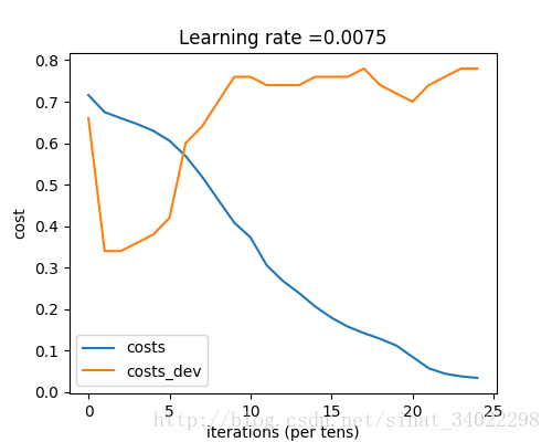
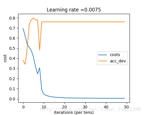
plt.plot(np.squeeze(costs))
plt.plot(np.squeeze(acc_dev))
plt.legend(["costs","acc_dev"],loc=0)
plt.ylabel('cost')
plt.xlabel('iterations (per tens)')
plt.title("Learning rate =" + str(learning_rate) )
plt.show()
return parameters
结果
根据课程设计了两个不同深度的神经网络,分别为:
layers_dims = [12288, 20, 7, 5, 1] # 5-layer model
layers_dims = [12288, 100, 20, 7, 5, 1] # 6-layer model