Building your Deep Neural Network: Step by Step
欢迎来到第四周作业(第二部分的第一部分)!您之前已经训练了一个两层的神经网络(只有一个隐藏层)。这周,你将构建一个深度神经网络,你想要多少层就有多少层!
•在本笔记本中,您将实现构建深度神经网络所需的所有功能(函数)。
•在下一个作业中,你将使用这些函数来建立一个用于图像分类的深度神经网络。
完成这项任务后,您将能够:
•使用非线性单元,比如ReLU来改进你的模型
•构建更深层次的神经网络(隐含层超过1层)
•实现一个易于使用的神经网络类
符号:
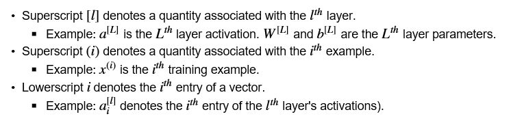
就是上标的【l】代表第l层,上标的【i】代表第i个样本,下标的 i 代表第 i 个条目
1 - Packages 包
让我们首先导入在此任务中需要的所有包。
·numpy是使用Python进行科学计算的主要包。
·matplotlib是一个用Python绘制图形的库。
·dnn_utils为本笔记本提供了一些必要的函数。
·testCases提供了一些测试用例来评估函数的正确性
·seed(1)用于保持所有随机函数调用的一致性。它将帮助我们批改你的作业。请不要换种子。
import numpy as np
import h5py #h5py是Python语言用来操作HDF5的模块。
import matplotlib.pyplot as plt
from testCases_v2 import *
from dnn_utils_v2 import sigmoid, sigmoid_backward, relu, relu_backward

%matplotlib inline
plt.rcParams['figure.figsize'] = (5.0, 4.0) # set default size of plots
plt.rcParams['image.interpolation'] = 'nearest'
plt.rcParams['image.cmap'] = 'gray'

%load_ext autoreload
%autoreload 2

np.random.seed(1)
python库——h5py入门讲解,来自neu_张康,链接:https://blog.csdn.net/csdn15698845876/article/details/73278120
%load_ext autoreload是什么意思:在执行用户代码前,重新装入 软件的扩展和模块。autoreload 意思是自动重新装入。它后面可带参数。参数意思你要查你自己的版本帮助文件。一般说:
无参:装入所有模块。
0:不执行 装入命令。
1: 只装入所有 %aimport 要装模块
2:装入所有 %aimport 不包含的模块。
2 - Outline of the Assignment(作业大纲)
要构建神经网络,您将实现几个“辅助函数”。这些辅助函数将用于下一个任务,以建立一个两层神经网络和一个L层神经网络。您将实现的每个小助手函数都有详细的说明,这些说明将指导您完成必要的步骤。这是这个作业的大纲,你会:
•初始化一个二层网络和一个L层神经网络的参数。
•实现转发模块(下图中用紫色显示)。
◾完成一层的线性部分的向前传播步骤(得到Z [l])
◾我们给你激活函数(relu /sigmoid)
◾将前两步骤组合成一个新的函数【线性- >激活转发】
◾堆栈(线性- > RELU)提出时间 L - 1 函数(通过L - 1层1)并添加一个(线性- >sigmoid),最后(最后一层L)。这将为您提供一个新的L_model_forward函数。
•计算损失。
•实现反向传播模块(下图中用红色表示)。
◾完成一层的向后传播的线性部分的步骤。
◾我们给你激活函数的梯度(relu_backward / sigmoid_backward)
◾将前两步骤组合成一个新的线性- >激活 反向功能。
◾堆栈(线性- > RELU)向后 并添加l - 1倍(线性- >乙状结肠)向后一个新的L_model_backward函数
•最后更新参数。
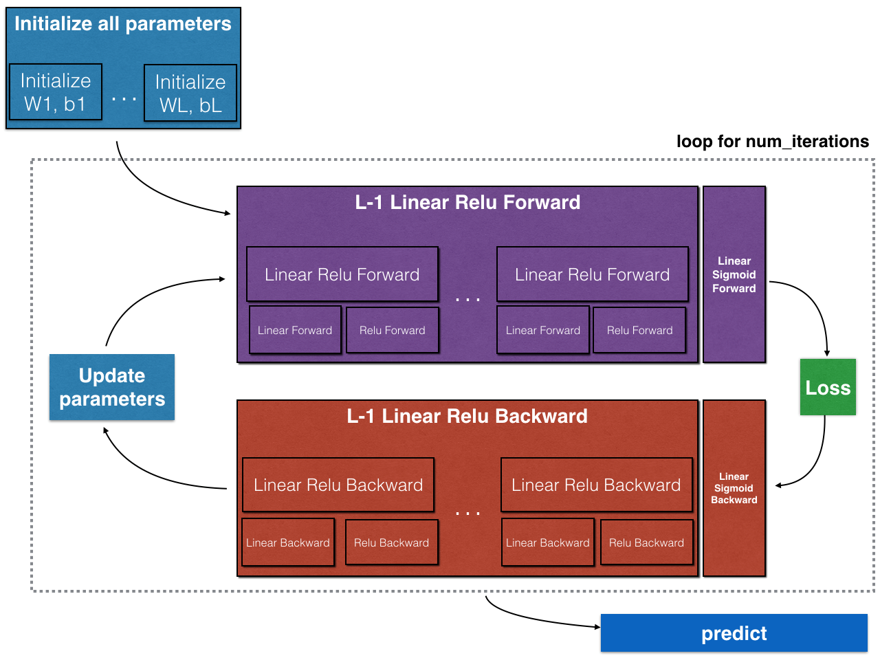
**Figure 1**
注意,对于每个前向函数,都有一个对应的后向函数。这就是为什么在向前(前向)模块的每一步都要在缓存中存储一些值。缓存的值对于计算梯度很有用。在反向传播模块中,您将使用缓存计算梯度。这个作业将确切地告诉你如何执行这些步骤中的每一步。
3 - Initialization 初始化
您将编写两个帮助函数来初始化模型的参数。第一个函数将用于初始化一个两层模型的参数。第二种方法将这个初始化过程推广到L层。
3.1 - 2-layer Neural Network(2层神经网络)
练习:创建并初始化两层神经网络的参数。
说明:
•模型结构为:LINEAR -> RELU -> LINEAR -> SIGMOID。
•对权重矩阵使用随机初始化。使用np.random.randn(shape)*0.01表示正确的形状。
•对偏差使用零初始化。使用np.zeros(形状)。


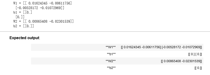
 1 # GRADED FUNCTION: initialize_parameters
 2
 3 def initialize_parameters(n_x, n_h, n_y):
 4     """
 5     Argument:
 6     n_x -- size of the input layer
 7     n_h -- size of the hidden layer
 8     n_y -- size of the output layer
 9
10     Returns:
11     parameters -- python dictionary containing your parameters:
12                     W1 -- weight matrix of shape (n_h, n_x)
13                     b1 -- bias vector of shape (n_h, 1)
14                     W2 -- weight matrix of shape (n_y, n_h)
15                     b2 -- bias vector of shape (n_y, 1)
16     """
17
18     np.random.seed(1)
19
20     ### START CODE HERE ### (≈ 4 lines of code)
21     W1 = np.random.randn(n_h, n_x)*0.01
22     b1 = np.zeros((n_h, 1))
23     W2 = np.random.randn(n_y, n_h)*0.01
24     b2 = np.zeros((n_y, 1))
25     ### END CODE HERE ###
26
27     assert(W1.shape == (n_h, n_x))
28     assert(b1.shape == (n_h, 1))
29     assert(W2.shape == (n_y, n_h))
30     assert(b2.shape == (n_y, 1))
31
32     parameters = {"W1": W1,
33                   "b1": b1,
34                   "W2": W2,
35                   "b2": b2}
36
37     return parameters
parameters = initialize_parameters(2,2,1)
print("W1 = " + str(parameters["W1"]))
print("b1 = " + str(parameters["b1"]))
print("W2 = " + str(parameters["W2"]))
print("b2 = " + str(parameters["b2"]))
结果:
3.2 - L-layer Neural Network L层的神经网络
更深的L层神经网络的初始化更加复杂,因为有更多的权值矩阵和偏差向量。在完成initialize_parameters_deep时,应该确保各层之间的维度匹配。回想一下,n [l]是 l 层中的单元数。例如,如果我们的输入X的大小是(12288,209)(m=209个例子)那么:

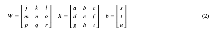
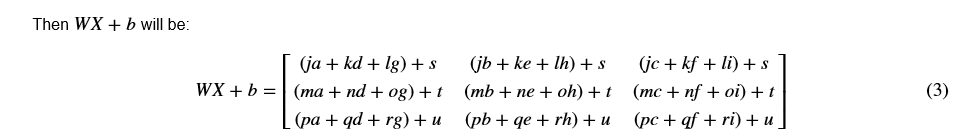
记住,当我们用python计算WX+b时,它执行广播机制 。例如,如果:
练习:实现L层神经网络的初始化。
说明:
•The model’s structure is [LINEAR -> RELU] × (L-1) -> LINEAR -> SIGMOID. I.e., it has L−1 layers using a ReLU activation function followed by an output layer with a sigmoid activation function.
•对权重矩阵使用随机初始化。使用np.random.rand(shape) * 0.01。
•对偏差使用零初始化。使用np.zeros(形状)。
•我们将存储n[l],不同层的单位数量,在一个变量layer_dims中。例如,上周的“平面数据分类模型”的layer_dims应该是[2,4,1]:有两个输入,一个隐含层有4个隐含单元,一个输出层有1个输出单元。即W1的形状为(4,2),b1为(4,1),W2为(1,4),b2为(1,1)。现在你可以将它推广到L层!
•这是L=1(一层神经网络)的实现。它会启发你实现一般情况(l层神经网络)。
if L == 1:
      parameters["W" + str(L)] = np.random.randn(layer_dims[1], layer_dims[0]) * 0.01
      parameters["b" + str(L)] = np.zeros((layer_dims[1], 1))
# GRADED FUNCTION: initialize_parameters_deep

def initialize_parameters_deep(layer_dims):
    """
    Arguments:
    layer_dims -- python array (list) containing the dimensions of each layer in our network

    Returns:
    parameters -- python dictionary containing your parameters "W1", "b1", ..., "WL", "bL":
                    Wl -- weight matrix of shape (layer_dims[l], layer_dims[l-1])
                    bl -- bias vector of shape (layer_dims[l], 1)
    """

    np.random.seed(3)
    parameters = {}
    L = len(layer_dims)            # number of layers in the network

    for l in range(1, L):
        ### START CODE HERE ### (≈ 2 lines of code)
        parameters['W' + str(l)] = np.random.randn(layer_dims[l], layer_dims[l-1]) * 0.01
        parameters['b' + str(l)] = np.zeros((layer_dims[l], 1))
        ### END CODE HERE ###

        assert(parameters['W' + str(l)].shape == (layer_dims[l], layer_dims[l-1]))
        assert(parameters['b' + str(l)].shape == (layer_dims[l], 1))


    return parameters
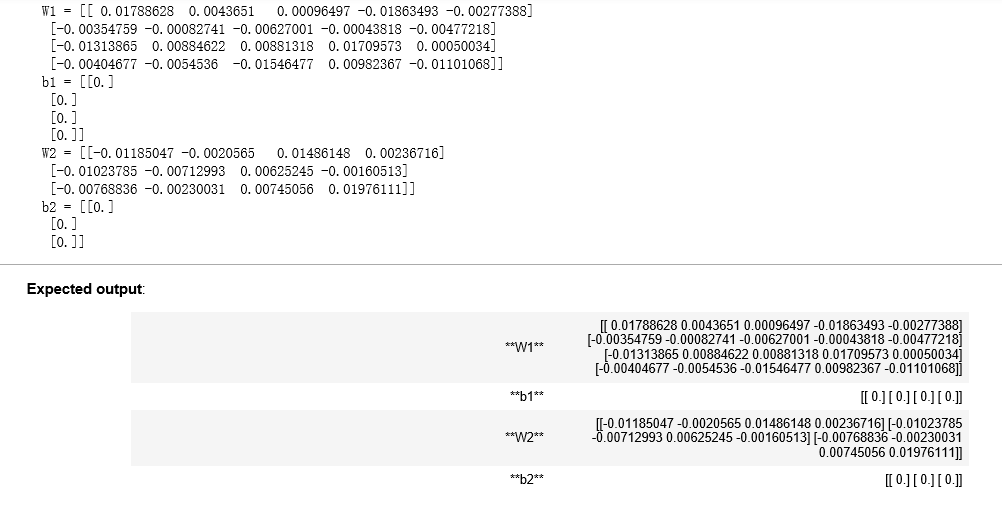
parameters = initialize_parameters_deep([5,4,3])
print("W1 = " + str(parameters["W1"]))
print("b1 = " + str(parameters["b1"]))
print("W2 = " + str(parameters["W2"]))
print("b2 = " + str(parameters["b2"]))
结果:
4 - Forward propagation module 前向传播模块
4.1 - Linear Forward 线性向前
现在您已经初始化了参数,您将实现向前传播模块。您将从实现一些基本功能开始,稍后在实现模型时将使用这些功能。您将按此顺序完成三个功能:
•线性
•线性->激活,其中激活为ReLU或Sigmoid。
•[LINEAR -> RELU] * (L-1) -> LINEAR -> SIGMOID(全模型)
线性向前模块(对所有例子进行矢量化)计算如下方程:Z [l] =W [l] A [l−1]+b [l] (4) 这里 A [0] =X
练习:建立正向传播的线性部分。
提示:该单位的数学表示为Z[l]=W[l]A[l−1]+b[l]。您可能还会发现np.dot()很有用。如果尺寸不匹配,打印W的形状可能会有所帮助。
# GRADED FUNCTION: linear_forward

def linear_forward(A, W, b):
    """
    Implement the linear part of a layer's forward propagation.

    Arguments:
    A -- activations from previous layer (or input data): (size of previous layer, number of examples)
    W -- weights matrix: numpy array of shape (size of current layer, size of previous layer)
    b -- bias vector, numpy array of shape (size of the current layer, 1)

    Returns:
    Z -- the input of the activation function, also called pre-activation parameter
    cache -- a python dictionary containing "A", "W" and "b" ; stored for computing the backward pass efficiently
    """

    ### START CODE HERE ### (≈ 1 line of code)
    Z = np.dot(W, A) + b
    ### END CODE HERE ###

    assert(Z.shape == (W.shape[0], A.shape[1]))
    cache = (A, W, b)

    return Z, cache
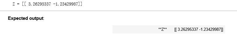
A, W, b = linear_forward_test_case()

Z, linear_cache = linear_forward(A, W, b)
print("Z = " + str(Z))
结果:
4.2 - Linear-Activation Forward 正向线性激活
在本笔记本中,您将使用两个激活函数:
Sigmoid:σ(Z) =σ(WA + b) =  。我们已经提供了sigmoid函数。这个函数返回两个项:激活值“a”和包含“Z”的“缓存”(我们将把它输入到相应的向后函数)。要使用它,你可以打称呼:
A, activation_cache = sigmoid(Z)
ReLU:ReLu的数学公式为A= ReLu (Z)=max(0,Z)。我们为您提供了relu功能。这个函数返回两个项:激活值“A”和包含“Z”的“缓存”(我们将把它输入到相应的向后函数)。要使用它,你可以打称:
A, activation_cache = relu(Z)
为了更方便,将两个函数(线性和激活)组合为一个函数(线性->激活)。因此,您将实现一个函数,它执行线性向前步骤,然后执行激活向前步骤。
Exercise:实现线性->激活层的正向传播。数学关系为:A[l]=g(Z[l])=g(W[l]A[l−1]+b[l]),其中活化“g”可以是sigmoid()或relu()。使用linear_forward()和正确的激活函数。
 1 # GRADED FUNCTION: linear_activation_forward
 2
 3 def linear_activation_forward(A_prev, W, b, activation):
 4     """
 5     Implement the forward propagation for the LINEAR->ACTIVATION layer
 6
 7     Arguments:
 8     A_prev -- activations from previous layer (or input data): (size of previous layer, number of examples)
 9     W -- weights matrix: numpy array of shape (size of current layer, size of previous layer)
10     b -- bias vector, numpy array of shape (size of the current layer, 1)
11     activation -- the activation to be used in this layer, stored as a text string: "sigmoid" or "relu"
12
13     Returns:
14     A -- the output of the activation function, also called the post-activation value
15     cache -- a python dictionary containing "linear_cache" and "activation_cache";
16              stored for computing the backward pass efficiently
17     """
18
19     if activation == "sigmoid":
20         # Inputs: "A_prev, W, b". Outputs: "A, activation_cache".
21         ### START CODE HERE ### (≈ 2 lines of code)
22         Z, linear_cache = linear_forward(A_prev, W, b) #前面linear_forward已经写好了
23         A, activation_cache = sigmoid(Z)
24         ### END CODE HERE ###
25
26     elif activation == "relu":
27         # Inputs: "A_prev, W, b". Outputs: "A, activation_cache".
28         ### START CODE HERE ### (≈ 2 lines of code)
29         Z, linear_cache = linear_forward(A_prev, W, b)
30         A, activation_cache = relu(Z)
31         ### END CODE HERE ###
32
33     assert (A.shape == (W.shape[0], A_prev.shape[1]))
34     cache = (linear_cache, activation_cache)
35
36     return A, cache
A_prev, W, b = linear_activation_forward_test_case()

A, linear_activation_cache = linear_activation_forward(A_prev, W, b, activation = "sigmoid")
print("With sigmoid: A = " + str(A))

A, linear_activation_cache = linear_activation_forward(A_prev, W, b, activation = "relu")
print("With ReLU: A = " + str(A))
结果:

注:在深度学习中,“[LINEAR->ACTIVATION]”计算在神经网络中被视为单层,而不是两层。
d) L-Layer Model 层数为L 的模型
在实现L层神经网络时,为了更加方便,您将需要一个函数复制前一个(RELU的linear_activation_forward) L−1倍,然后再使用一个SIGMOID的linear_activation_forward。
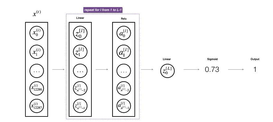
**Figure 2** : *[LINEAR -> RELU]
练习:实现上述模型的正向传播。
指令:在下面的代码中,变量AL将表示A [L]=σ(Z[L])=σ(W[L]A[L−1]+b[L]).有时候这也叫Yhat
提示:
•使用之前编写的函数
•使用for循环复制[LINEAR->RELU] (L-1)次
•不要忘记跟踪“缓存”列表中的缓存。要向列表添加新值c,可以使用list.append(c)。
 1 # GRADED FUNCTION: L_model_forward
 2
 3 def L_model_forward(X, parameters):
 4     """
 5     Implement forward propagation for the [LINEAR->RELU]*(L-1)->LINEAR->SIGMOID computation
 6
 7     Arguments:
 8     X -- data, numpy array of shape (input size, number of examples)
 9     parameters -- output of initialize_parameters_deep()
10
11     Returns:
12     AL -- last post-activation value
13     caches -- list of caches containing:
14                 every cache of linear_relu_forward() (there are L-1 of them, indexed from 0 to L-2)
15                 the cache of linear_sigmoid_forward() (there is one, indexed L-1)
16     """
17
18     caches = []
19     A = X
20     L = len(parameters) // 2                  # number of layers in the neural network
21
22     # Implement [LINEAR -> RELU]*(L-1). Add "cache" to the "caches" list.
23     for l in range(1, L):
24         A_prev = A
25         ### START CODE HERE ### (≈ 2 lines of code)
26         A, cache = linear_activation_forward(A_prev, parameters['W' + str(l)], parameters['b'+str(l)], activation = "relu")
27         caches.append(cache)
28
29         ### END CODE HERE ###
30
31     # Implement LINEAR -> SIGMOID. Add "cache" to the "caches" list.
32     ### START CODE HERE ### (≈ 2 lines of code)
33     AL, cache = linear_activation_forward(A, parameters['W'+str(L)], parameters['b'+str(L)], activation = "sigmoid")
34     caches.append(cache)
35     ### END CODE HERE ###
36
37     assert(AL.shape == (1,X.shape[1]))
38
39     return AL, caches
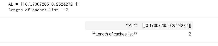
X, parameters = L_model_forward_test_case()
AL, caches = L_model_forward(X, parameters)
print("AL = " + str(AL))
print("Length of caches list = " + str(len(caches)))
结果:
太棒了!现在您有了一个完全的正向传播,它接受输入X并输出包含您的预测的行向量a [L]。它还记录了“缓存”中的所有中间值。使用A[L],您可以计算您的预测的成本。
5- Cost function 成本函数
现在您将实现向前和向后传播。你需要计算成本,因为你想检查你的模型是否真的在学习。
练习:计算交叉熵代价J,公式如下:

 1 # GRADED FUNCTION: compute_cost
 2
 3 def compute_cost(AL, Y):
 4     """
 5     Implement the cost function defined by equation (7).
 6
 7     Arguments:
 8     AL -- probability vector corresponding to your label predictions, shape (1, number of examples)
 9     Y -- true "label" vector (for example: containing 0 if non-cat, 1 if cat), shape (1, number of examples)
10
11     Returns:
12     cost -- cross-entropy cost
13     """
14
15     m = Y.shape[1]
16
17     # Compute loss from aL and y.
18     ### START CODE HERE ### (≈ 1 lines of code)
19     cost = (-1 / m) * np.sum(Y * np.log(AL) + (1 - Y) * np.log(1 - AL), axis = 1, keepdims = True)
20     ### END CODE HERE ###
21
22     cost = np.squeeze(cost)      # To make sure your cost's shape is what we expect (e.g. this turns [[17]] into 17).
23     assert(cost.shape == ())
24
25     return cost
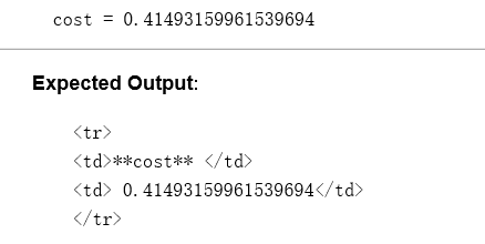
Y, AL = compute_cost_test_case()

print("cost = " + str(compute_cost(AL, Y)))
结果:
6 - Backward propagation module 反向传播模块
与前向传播一样,您将实现用于后向传播的辅助函数。记住,反向传播是用来计算关于参数的损失函数的梯度。
提示:

**Figure 3** : Forward and Backward propagation for *LINEAR->RELU->LINEAR->SIGMOID*
*紫色块表示正向传播,红色块表示反向传播
现在,与前向传播类似,您将通过三个步骤构建向后传播:
•线性向后
•线性->激活逆向,激活计算ReLU或Sigmoid激活的导数
•[LINEAR -> RELU] * (L-1) -> LINEAR -> SIGMOID - backward(整个模型)
6.1 - Linear backward 线性向后
对于第 l 层,线性部分就是:Z [l] =W [l] A [l−1] +b [l] (然后是激活)
假设已经求出了导数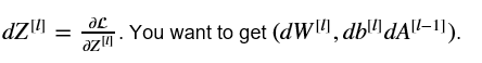 ,
,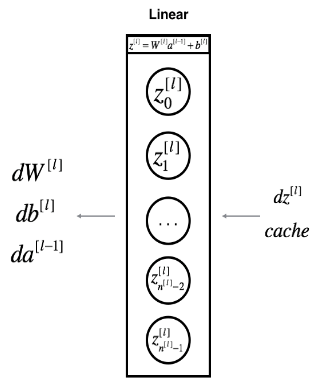
**Figure 4**
使用输入dZ [l]计算三个输出(dW [l]、db [l]、dA [l])。以下是你需要的公式:
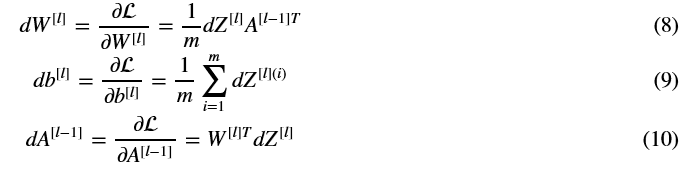
练习:使用上面的3个公式来实现linear_backward()。
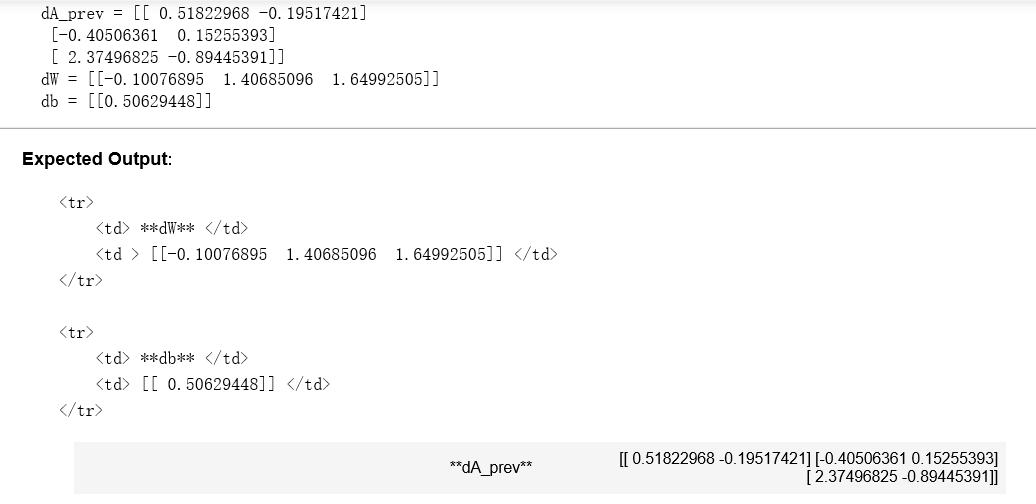
 1 # GRADED FUNCTION: linear_backward
 2
 3 def linear_backward(dZ, cache):
 4     """
 5     Implement the linear portion of backward propagation for a single layer (layer l)
 6
 7     Arguments:
 8     dZ -- Gradient of the cost with respect to the linear output (of current layer l)
 9     cache -- tuple of values (A_prev, W, b) coming from the forward propagation in the current layer
10
11     Returns:
12     dA_prev -- Gradient of the cost with respect to the activation (of the previous layer l-1), same shape as A_prev
13     dW -- Gradient of the cost with respect to W (current layer l), same shape as W
14     db -- Gradient of the cost with respect to b (current layer l), same shape as b
15     """
16     A_prev, W, b = cache
17     m = A_prev.shape[1]
18
19     ### START CODE HERE ### (≈ 3 lines of code)
20     dW = 1 / m * np.dot(dZ, A_prev.T)
21     db = 1 / m * np.sum(dZ, axis = 1, keepdims = True)
22     dA_prev = np.dot(W.T, dZ)
23     ### END CODE HERE ###
24
25     assert (dA_prev.shape == A_prev.shape)
26     assert (dW.shape == W.shape)
27     assert (db.shape == b.shape)
28
29     return dA_prev, dW, db
# Set up some test inputs
dZ, linear_cache = linear_backward_test_case()

dA_prev, dW, db = linear_backward(dZ, linear_cache)
print ("dA_prev = "+ str(dA_prev))
print ("dW = " + str(dW))
print ("db = " + str(db))
结果:
6.2 - Linear-Activation backward 向后的线性激活
接下来,您将创建一个合并两个辅助函数的函数:linear_backward和激活linear_activation_backward的后退步骤。
为了帮助你实现linear_activation_backward,我们提供了两个向后的函数:
sigmoid_backward:实现了SIGMOID单元的向后传播。你可以这样叫它:
dZ = sigmoid_backward(dA, activation_cache)
relu_backward:实现RELU单元的向后传播。你可以这样叫它:
dZ = relu_backward(dA, activation_cache)
如果g(.)是激活函数,则sigmoid_backward和relu_backward 计算的就是:
练习:实现线性>激活层的反向传播。
# GRADED FUNCTION: linear_activation_backward

def linear_activation_backward(dA, cache, activation):
    """
    Implement the backward propagation for the LINEAR->ACTIVATION layer.

    Arguments:
    dA -- post-activation gradient for current layer l
    cache -- tuple of values (linear_cache, activation_cache) we store for computing backward propagation efficiently
    activation -- the activation to be used in this layer, stored as a text string: "sigmoid" or "relu"

    Returns:
    dA_prev -- Gradient of the cost with respect to the activation (of the previous layer l-1), same shape as A_prev
    dW -- Gradient of the cost with respect to W (current layer l), same shape as W
    db -- Gradient of the cost with respect to b (current layer l), same shape as b
    """
    linear_cache, activation_cache = cache

    if activation == "relu":
        ### START CODE HERE ### (≈ 2 lines of code)
        dZ = relu_backward(dA, activation_cache)
        dA_prev, dW, db = linear_backward(dZ, linear_cache)
        ### END CODE HERE ###

    elif activation == "sigmoid":
        ### START CODE HERE ### (≈ 2 lines of code)
        dZ = sigmoid_backward(dA, activation_cache)
        dA_prev, dW, db = linear_backward(dZ, linear_cache)
        ### END CODE HERE ###

    return dA_prev, dW, db
AL, linear_activation_cache = linear_activation_backward_test_case()

dA_prev, dW, db = linear_activation_backward(AL, linear_activation_cache, activation = "sigmoid")
print ("sigmoid:")
print ("dA_prev = "+ str(dA_prev))
print ("dW = " + str(dW))
print ("db = " + str(db) + "\n")

dA_prev, dW, db = linear_activation_backward(AL, linear_activation_cache, activation = "relu")
print ("relu:")
print ("dA_prev = "+ str(dA_prev))
print ("dW = " + str(dW))
print ("db = " + str(db))
结果:

6.3 - L-Model Backward 有L层的向后模型
现在您将为整个网络实现反向函数。回想一下,在实现L_model_forward函数时,在每次迭代中存储一个包含(X、W、b和z)的缓存。因此,在L_model_backward函数中,您将从层L开始向后迭代所有隐藏层。在每一步中,您将使用层 l 的缓存值反向传播到层 l。下面的图5显示了反向传递。
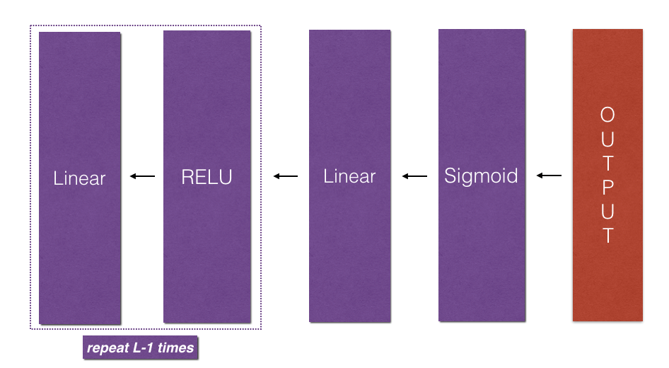
**Figure 5** : Backward pass
**初始化反向传播**:要通过这个网络反向传播,我们知道输出是,A [L] =σ(Z [L] ). 因此,您的代码需要计算dAL =  要做到这一点,使用这个公式(由微积分推导,你不需要深入的知识):
dAL = - (np.divide(Y, AL) - np.divide(1 - Y, 1 - AL)) # derivative of cost with respect to AL
然后你可以使用激活后梯度dAL继续向后移动。如图5所示,现在可以将dAL输入到您实现的LINEAR->SIGMOID向后函数中(它将使用L_model_forward函数存储的缓存值)。在此之后,您将必须使用一个for循环来使用LINEAR->RELU backward函数迭代所有其他层。应该将每个dA、dW和db存储在梯度字典中。为此,使用以下公式:

例如,对于l=3,这将在梯度[“dW3”]中存储dW [l]。
练习:实现[LINEAR->RELU] * (L-1) -> LINEAR-> SIGMOID模型的反向传播。
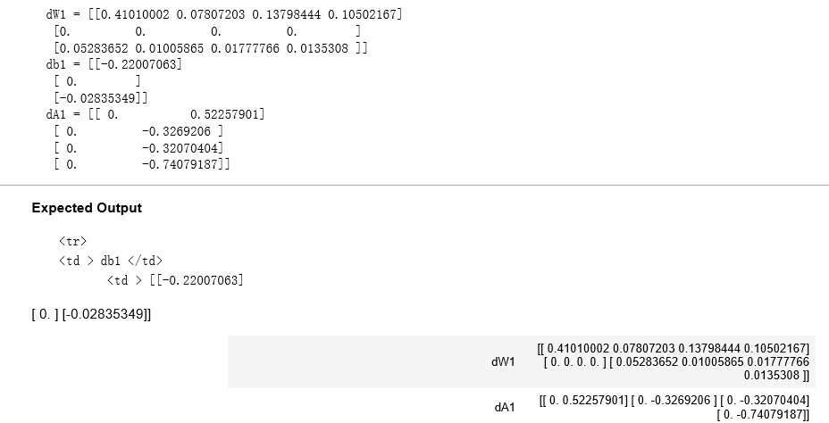
 1 # GRADED FUNCTION: L_model_backward
 2
 3 def L_model_backward(AL, Y, caches):
 4     """
 5     Implement the backward propagation for the [LINEAR->RELU] * (L-1) -> LINEAR -> SIGMOID group
 6
 7     Arguments:
 8     AL -- probability vector, output of the forward propagation (L_model_forward())
 9     Y -- true "label" vector (containing 0 if non-cat, 1 if cat)
10     caches -- list of caches containing:
11                 every cache of linear_activation_forward() with "relu" (it's caches[l], for l in range(L-1) i.e l = 0...L-2)
12                 the cache of linear_activation_forward() with "sigmoid" (it's caches[L-1])
13
14     Returns:
15     grads -- A dictionary with the gradients
16              grads["dA" + str(l)] = ...
17              grads["dW" + str(l)] = ...
18              grads["db" + str(l)] = ...
19     """
20     grads = {}
21     L = len(caches) # the number of layers 求出层数 前L-2个是“relu”,第L-1层是“sigmoid”
22     m = AL.shape[1] #样本数
23     Y = Y.reshape(AL.shape) # after this line, Y is the same shape as AL 使Y和AL的形状一样
24
25     # Initializing the backpropagation
26     ### START CODE HERE ### (1 line of code)
27     dAL = - (np.divide(Y, AL) - np.divide(1 - Y, 1 - AL))
28     ### END CODE HERE ###
29
30     # Lth layer (SIGMOID -> LINEAR) gradients. Inputs: "AL, Y, caches". Outputs: "grads["dAL"], grads["dWL"], grads["dbL"]
31     #这边是第L层,就是最后一层,使用的是sigmiod激活函数
32     ### START CODE HERE ### (approx. 2 lines)
33     current_cache = caches[L - 1]
34     grads["dA" + str(L)], grads["dW" + str(L)], grads["db" + str(L)] = linear_activation_backward(dAL, current_cache, activation = "sigmoid")
35     ### END CODE HERE ###
36
37     for l in reversed(range(L - 1)):
38         # lth layer: (RELU -> LINEAR) gradients.
39         # Inputs: "grads["dA" + str(l + 2)], caches". Outputs: "grads["dA" + str(l + 1)] , grads["dW" + str(l + 1)] , grads["db" + str(l + 1)]
40         ### START CODE HERE ### (approx. 5 lines)
41         current_cache = caches[l]
42         dA_prev_temp, dW_temp, db_temp = linear_activation_backward(grads["dA" + str(l + 2)], current_cache, activation = "relu")
43         grads["dA" + str(l + 1)] = dA_prev_temp
44         grads["dW" + str(l + 1)] = dW_temp
45         grads["db" + str(l + 1)] = db_temp
46         ### END CODE HERE ###
47
48     return grads
AL, Y_assess, caches = L_model_backward_test_case()
grads = L_model_backward(AL, Y_assess, caches)
print ("dW1 = "+ str(grads["dW1"]))
print ("db1 = "+ str(grads["db1"]))
print ("dA1 = "+ str(grads["dA1"]))
结果:
6.4 - Update Parameters 更新参数
在本节中,你将使用梯度下降更新模型的参数:

这是 α 是学习速率,计算更新后的参数后,将它们存储在参数字典中。
练习:实现update_parameters()来使用梯度下降更新参数。
说明:对于l=1,2,…,l,每个W [l]和b [l]使用梯度下降更新参数。
 1 # GRADED FUNCTION: update_parameters
 2
 3 def update_parameters(parameters, grads, learning_rate):
 4     """
 5     Update parameters using gradient descent
 6
 7     Arguments:
 8     parameters -- python dictionary containing your parameters
 9     grads -- python dictionary containing your gradients, output of L_model_backward
10
11     Returns:
12     parameters -- python dictionary containing your updated parameters
13                   parameters["W" + str(l)] = ...
14                   parameters["b" + str(l)] = ...
15     """
16
17     L = len(parameters) // 2 # number of layers in the neural network 因为这里参数是成对出现的eg:W1,b1
18
19     # Update rule for each parameter. Use a for loop.
20     ### START CODE HERE ### (≈ 3 lines of code)
21     for l in range(L):
22         parameters["W" + str(l+1)] = parameters["W" + str(l+1)] - learning_rate * grads["dW" + str(l + 1)]
23         parameters["b" + str(l+1)] = parameters["b" + str(l+1)] - learning_rate * grads["db" + str(l + 1)]
24     ### END CODE HERE ###
25
26     return parameters
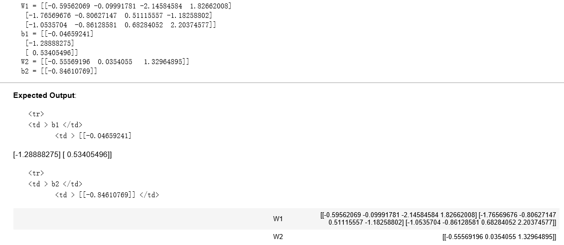
parameters, grads = update_parameters_test_case()
parameters = update_parameters(parameters, grads, 0.1)

print ("W1 = "+ str(parameters["W1"]))
print ("b1 = "+ str(parameters["b1"]))
print ("W2 = "+ str(parameters["W2"]))
print ("b2 = "+ str(parameters["b2"]))
结果:
7 - Conclusion 结论
祝贺您实现了构建深度神经网络所需的所有功能!
我们知道这是一个漫长的任务,但如果继续前进,情况只会越来越好。作业的下一部分比较容易。
在下一个作业中,你将把所有这些放在一起来建立两个模型:
A two-layer neural network
An L-layer neural network
实际上,您将使用这些模型来分类猫和非猫的图像!