课程笔记

算法将一幅图片分为内容+风格，有了这两像，图片也就确定了，所以”生成图片主要的思想，通过两个损失函数（内容损失+风格损失）来进行迭代更新”
这里写图片描述

迁移学习总体分为三步:

建立内容损失函数 $J_{content}(C,G)$
建立风格损失函数 $J_{style}(S,G)$
加权组合起来，即总体损失函数 $J(G) = \alpha J_{content}(C,G) + \beta J_{style}(S,G)$ .

CNN是对输入的图片进行处理的神经网络，一般有卷积层、池化层、全连接层，每一层都是对图片进行像素级的运算。图片以矩阵的形式输入神经网络，在经过每一层时的输出依然时矩阵，把这个矩阵反转回去得到的图像，就是这一层对图片进行处理后得到的图像。

一个神经网络，前面几层（浅层）一般检测图片的基础特征，例如边缘和结构；后面几层（深层）一般检测图片的综合特征，例如具体的类别。

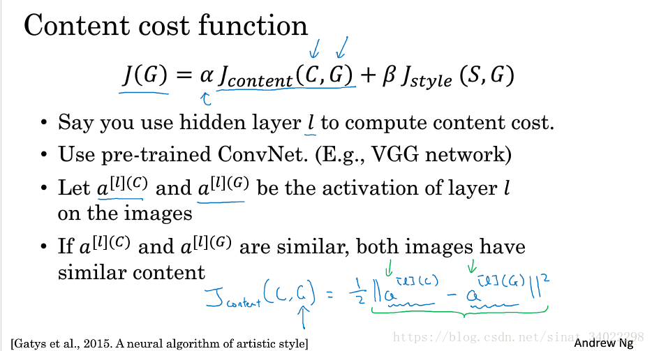
内容损失函数

我们希望“生成的”图像G具有与输入图像C相似的内容。但是选择神经网络的哪些层的输出来表示图片的内容呢，作业中使用了中间的层，既不太浅也不太深，可以取得好的效果。（完成此练习后，请随时返回并尝试使用不同的图层，以查看结果的变化。）

使用已经训练过的网络 VGG，输出层输入图像为C，经过VGG网络前向传播，得到 $[l]$ 层输出为 $a^{[l](C)}$ ，这里用 $a^{(C)}$ 表示；同时生成一张白噪声的图片G，重复同样的操作得到 $a^{(G)}$ ，从而可以得到内容损失函数：

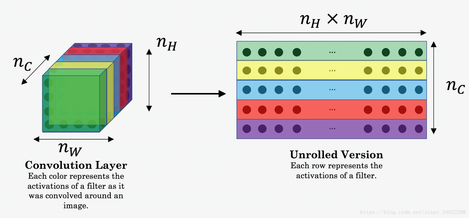
\begin{matrix} (1) & J_{c o n t e n t} (C, G) = \frac{1}{4 \times n_{H} \times n_{W} \times n_{C}} \sum_{all entries} (a^{(C)} - a^{(G)})^{2} \end{matrix}

$J_{content}(C,G) = \frac{1}{4 \times n_H \times n_W \times n_C}\sum _{ \text{all entries}} (a^{(C)} - a^{(G)})^2\tag{1}$

$n_H, n_W$ and $n_C$ 时指定神经网络层的输出矩阵，这里为了方便计算，做举证展开（Unrolled），如下图：
这里写图片描述

What you should remember:
- The content cost takes a hidden layer activation of the neural network, and measures how different $a^{(C)}$ and $a^{(G)}$ are.
- When we minimize the content cost later, this will help make sure $G$ has similar content as $C$ .

风格损失函数

上面的内容矩阵是直接采用指定层的输出矩阵，而风格矩阵在这里用 “Gram matrix.” 表示，也叫相关矩阵，如下图：

计算Gram Matrix首先对矩阵进行展开（Unrolled），随后再进行矩阵转置，矩阵点乘。
这里写图片描述
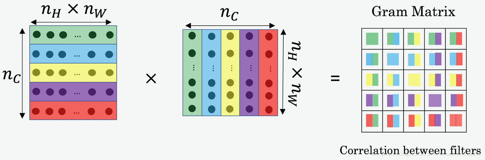
在线性代数中， Gram matrix表示的是矩阵中不同向量之间的相关性， G 的向量是做如下运算得到的：

G_{i j} = v_{i}^{T} v_{j} = n p . d o t (v_{i}, v_{j})

$G_{ij} = v_{i}^T v_{j} = np.dot(v_{i}, v_{j})$ .
矩阵对角线上的元素是 向量内积；非对角线元素是 两两不同向量内积，值的大小可以反应这两个不同向量的相关性，值越大，相关性越大。

在神经网络中，上述的进过 Unrolled 矩阵的不同向量代表同一层不同滤波器的输出，所以 Gram Matrix 对角线上的元素 $G_{ii}$ 衡量该滤波器检测的特征值在图片中所占的比例；例如，di $i$ 层卷积检测垂直结构，则 $G_{ii}$ 可以衡量该图片中垂直结构所占比例的大小。而 $G_{ij}$ 衡量不同滤波器的相似程度。笔者认为风格函数的主要贡献在 Gram Matrix 对角线。

在有了 Gram Matrix 以后，风格损失函数定义如下：

\begin{matrix} (2) & J_{s t y l e}^{[l]} (S, G) = \frac{1}{4 \times {n_{C}}^{2} \times (n_{H} \times n_{W})^{2}} \sum_{i = 1}^{n_{C}} \sum_{j = 1}^{n_{C}} (G_{i j}^{(S)} - G_{i j}^{(G)})^{2} \end{matrix}

$J_{style}^{[l]}(S,G) = \frac{1}{4 \times {n_C}^2 \times (n_H \times n_W)^2} \sum _{i=1}^{n_C}\sum_{j=1}^{n_C}(G^{(S)}_{ij} - G^{(G)}_{ij})^2\tag{2}$

What you should remember:
- The style of an image can be represented using the Gram matrix of a hidden layer’s activations. However, we get even better results combining this representation from multiple different layers. This is in contrast to the content representation, where usually using just a single hidden layer is sufficient.
- Minimizing the style cost will cause the image $G$ to follow the style of the image $S$ .

总体损失函数

最后，将内容损失函数和风格损失函数进行加权相加，得到总的损失函数：

J (G) = α J_{c o n t e n t} (C, G) + β J_{s t y l e} (S, G)

$J(G) = \alpha J_{content}(C,G) + \beta J_{style}(S,G)$

有了总体损失函数，每次迭代更新的参数应该是输入白噪声图片的像素；就像是神经网络看了两幅画，找到他们的特征（ $[l]$ 层输出图像），然后找到不同的地方（总体损失函数），去做修正（像素级），最终得到想要的结果。具体怎么更新图片像素，有待研究。

pycharm版程序

使用 tensorflow 进行训练

import os
import sys
import scipy.io
import scipy.misc
import matplotlib.pyplot as plt
from matplotlib.pyplot import imshow
from PIL import Image
from nst_utils import *
import numpy as np
import tensorflow as tf

import datetime


# GRADED FUNCTION: compute_content_cost
def compute_content_cost(a_C, a_G):
    """
    Computes the content cost

    Arguments:
    a_C -- tensor of dimension (1, n_H, n_W, n_C), hidden layer activations representing content of the image C
    a_G -- tensor of dimension (1, n_H, n_W, n_C), hidden layer activations representing content of the image G

    Returns:
    J_content -- scalar that you compute using equation 1 above.
    """

    ### START CODE HERE ###
    # Retrieve dimensions from a_G (≈1 line)
    m, n_H, n_W, n_C = a_G.get_shape().as_list()                # 用 a_G 和 a_C 的区别?

    # Reshape a_C and a_G (≈2 lines)
    a_C_unrolled = tf.reshape(a_C,[n_H * n_W, n_C])
    a_G_unrolled = tf.reshape(a_G,[n_H * n_W, n_C])

    # compute the cost with tensorflow (≈1 line)
    J_content = tf.reduce_sum(tf.square(tf.subtract(a_C_unrolled, a_G_unrolled))) / (4*n_H*n_W*n_C)
    ### END CODE HERE ###

    return J_content


# GRADED FUNCTION: gram_matrix
def gram_matrix(A):
    """
    Argument:
    A -- matrix of shape (n_C, n_H*n_W)

    Returns:
    GA -- Gram matrix of A, of shape (n_C, n_C)
    """

    ### START CODE HERE ### (≈1 line)
    GA = tf.matmul(A, A ,transpose_a=False, transpose_b=True)       # 矩阵相乘,后面的flag表示是否对对应矩阵进行转置操作
    ### END CODE HERE ###

    return GA


# GRADED FUNCTION: compute_layer_style_cost
def compute_layer_style_cost(a_S, a_G):
    """
    Arguments:
    a_S -- tensor of dimension (1, n_H, n_W, n_C), hidden layer activations representing style of the image S
    a_G -- tensor of dimension (1, n_H, n_W, n_C), hidden layer activations representing style of the image G

    Returns:
    J_style_layer -- tensor representing a scalar value, style cost defined above by equation (2)
    """

    ### START CODE HERE ###
    # Retrieve dimensions from a_G (≈1 line)
    m, n_H, n_W, n_C = a_G.get_shape().as_list()

    # Reshape the images to have them of shape (n_H*n_W, n_C) (≈2 lines)
    a_S = tf.reshape(a_S, [n_W*n_H, n_C])
    a_G = tf.reshape(a_G, [n_W*n_H, n_C])

    # Computing gram_matrices for both images S and G (≈2 lines)
    GS = gram_matrix(tf.transpose(a_S))
    GG = gram_matrix(tf.transpose(a_G))
    # GS = gram_matrix(a_S)
    # GG = gram_matrix(a_G)

    # Computing the loss (≈1 line)
    J_style_layer = tf.reduce_sum(tf.square(tf.subtract(GS, GG))) / (4*tf.to_float(tf.square(n_C*n_H*n_W)))

    ### END CODE HERE ###

    return J_style_layer


def compute_style_cost(model, STYLE_LAYERS):
    """
    Computes the overall style cost from several chosen layers

    Arguments:
    model -- our tensorflow model
    STYLE_LAYERS -- A python list containing:
                        - the names of the layers we would like to extract style from
                        - a coefficient for each of them

    Returns:
    J_style -- tensor representing a scalar value, style cost defined above by equation (2)
    """

    # initialize the overall style cost
    J_style = 0

    for layer_name, coeff in STYLE_LAYERS:
        # Select the output tensor of the currently selected layer
        out = model[layer_name]

        # Set a_S to be the hidden layer activation from the layer we have selected, by running the session on out
        a_S = sess.run(out)

        # Set a_G to be the hidden layer activation from same layer. Here, a_G references model[layer_name]
        # and isn't evaluated yet. Later in the code, we'll assign the image G as the model input, so that
        # when we run the session, this will be the activations drawn from the appropriate layer, with G as input.
        a_G = out

        # Compute style_cost for the current layer
        J_style_layer = compute_layer_style_cost(a_S, a_G)

        # Add coeff * J_style_layer of this layer to overall style cost
        J_style += coeff * J_style_layer

    return J_style


# GRADED FUNCTION: total_cost
def total_cost(J_content, J_style, alpha=10, beta=40):
    """
    Computes the total cost function

    Arguments:
    J_content -- content cost coded above
    J_style -- style cost coded above
    alpha -- hyperparameter weighting the importance of the content cost
    beta -- hyperparameter weighting the importance of the style cost

    Returns:
    J -- total cost as defined by the formula above.
    """

    ### START CODE HERE ### (≈1 line)
    J = alpha * J_content + beta * J_style
    ### END CODE HERE ###

    return J


def model_nn(sess, input_image, num_iterations=200):
    # Initialize global variables (you need to run the session on the initializer)
    ### START CODE HERE ### (1 line)
    sess.run(tf.global_variables_initializer())
    ### END CODE HERE ###

    # Run the noisy input image (initial generated image) through the model. Use assign().
    ### START CODE HERE ### (1 line)
    sess.run(model['input'].assign(input_image))
    ### END CODE HERE ###

    for i in range(num_iterations):

        # Run the session on the train_step to minimize the total cost
        ### START CODE HERE ### (1 line)
        sess.run(train_step)
        ### END CODE HERE ###

        # Compute the generated image by running the session on the current model['input']
        ### START CODE HERE ### (1 line)
        generated_image = sess.run(model['input'])
        ### END CODE HERE ###

        # Print every 20 iteration.
        if i % 20 == 0:
            Jt, Jc, Js = sess.run([J, J_content, J_style])
            print("Iteration " + str(i) + " :")
            print("total cost = " + str(Jt))
            print("content cost = " + str(Jc))
            print("style cost = " + str(Js))

            # save current generated image in the "/output" directory
            save_image("out1/3/" + str(i) + ".png", generated_image)

    # save last generated image
    save_image('out1/3/generated_image.jpg', generated_image)

    return generated_image




if __name__ == '__main__':

    starttime = datetime.datetime.now()

    ###############################################
    # Reset the graph
    tf.reset_default_graph()

    # Start interactive session
    sess = tf.InteractiveSession()
    content_image = scipy.misc.imread("input/y.jpg")

    content_image = reshape_and_normalize_image(content_image)

    style_image = scipy.misc.imread("images/sky.jpg")
    style_image = reshape_and_normalize_image(style_image)

    generated_image = generate_noise_image(content_image)
    plt.imshow(generated_image[0])
    plt.show()

    model = load_vgg_model("pretrained-model/imagenet-vgg-verydeep-19.mat")

    STYLE_LAYERS = [                                     # style_layers 的作用
        ('conv1_1', 0.2),
        ('conv2_1', 0.2),
        ('conv3_1', 0.2),
        ('conv4_1', 0.2),
        ('conv5_1', 0.2)]

    # Assign the content image to be the input of the VGG model.
    sess.run(model['input'].assign(content_image))

    # Select the output tensor of layer conv4_2
    out = model['conv4_2']

    # Set a_C to be the hidden layer activation from the layer we have selected
    a_C = sess.run(out)

    # Set a_G to be the hidden layer activation from same layer. Here, a_G references model['conv4_2']
    # and isn't evaluated yet. Later in the code, we'll assign the image G as the model input, so that
    # when we run the session, this will be the activations drawn from the appropriate layer, with G as input.
    a_G = out

    # Compute the content cost
    J_content = compute_content_cost(a_C, a_G)

    # Assign the input of the model to be the "style" image
    sess.run(model['input'].assign(style_image))

    # Compute the style cost
    J_style = compute_style_cost(model, STYLE_LAYERS)

    ### START CODE HERE ### (1 line)
    J = total_cost(J_content=J_content, J_style=J_style)
    ### END CODE HERE ###

    # define optimizer (1 line)
    optimizer = tf.train.AdamOptimizer(2.0)

    # define train_step (1 line)
    train_step = optimizer.minimize(J)

    model_nn(sess, generated_image)

    #################################################
    endtime = datetime.datetime.now()
    print("the running time :" + str((endtime - starttime).seconds))
    print("END!")

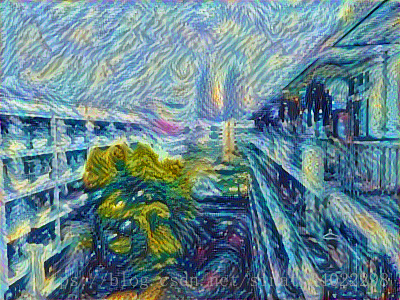
结果

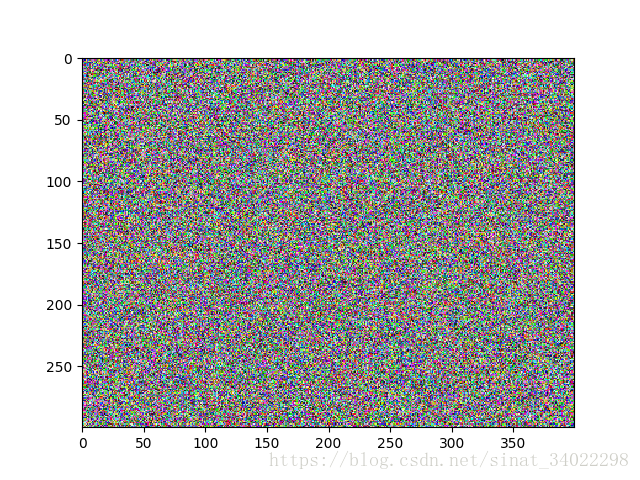
刚开始生成的白噪声图片，400*300 ，神经网络通过学习，把这个图片改成想要的模样，可怕：
这里写图片描述

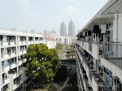
内容图片（400*300）：
这里写图片描述

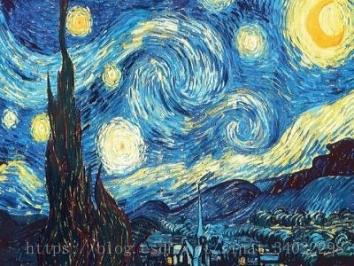
风格图片（400*300）：
这里写图片描述

生成图片（400*300），迭代200，结果已稳定：
这里写图片描述

《深度学习——Andrew Ng》第四课第四周编程作业_2_神经网络风格迁移

课程笔记

内容损失函数

风格损失函数

总体损失函数

pycharm版程序

结果

猜你喜欢