SVM分类,就是找到一个平面,让两个分类集合的支持向量或者所有的数据(LSSVM)离分类平面最远;
SVR回归,就是找到一个回归平面,让一个集合的所有数据到该平面的距离最近。
SVR是支持向量回归(support vector regression)的英文缩写,是支持向量机(SVM)的重要的应用分支。
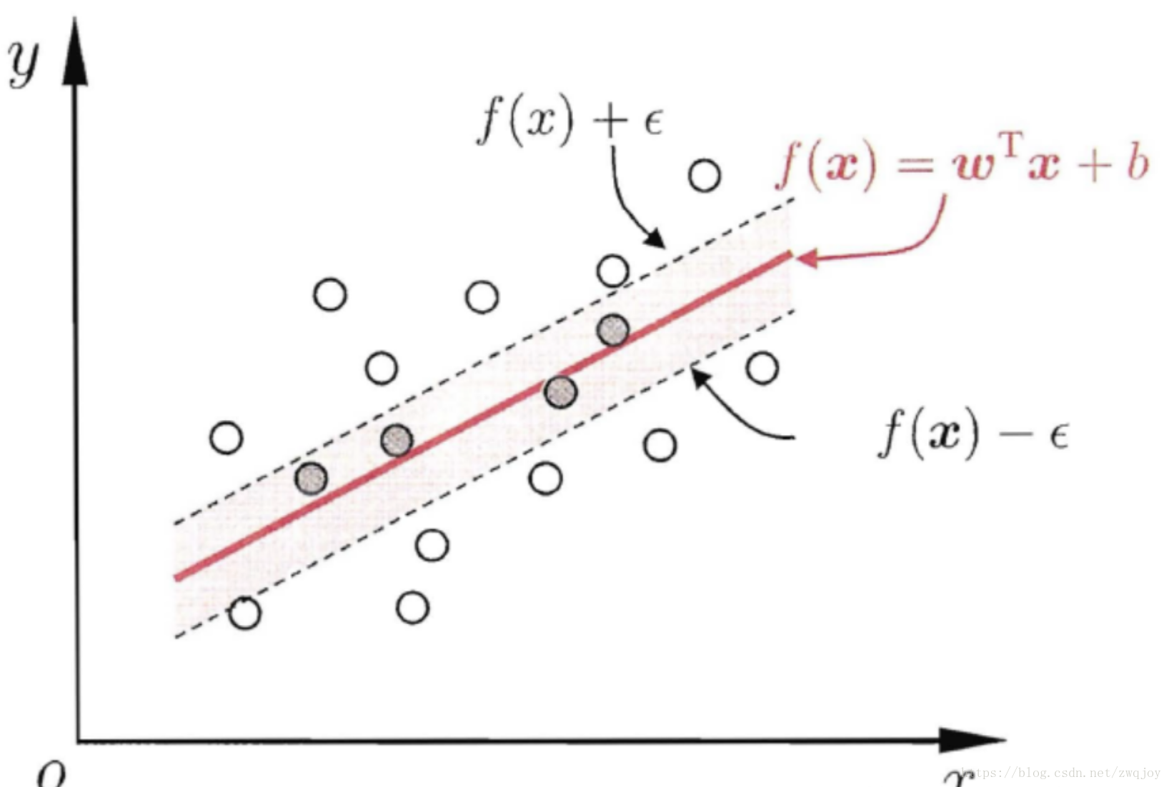
传统回归方法当且仅当回归f(x)完全等于y时才认为预测正确,如线性回归中常用(f(x)−y)2来计算其损失。
而支持向量回归则认为只要f(x)与y偏离程度不要太大,既可以认为预测正确,不用计算损失,具体的,就是设置阈值α,只计算|f(x)−y|>α的数据点的loss,如下图所示,阴影部分的数据点我们都认为该模型预测准确了,只计算阴影外的数据点的loss:
数据处理
preprocessing.scale()作用:
scale()是用来对原始样本进行缩放的,范围可以自己定,一般是[0,1]或[-1,1]。
缩放的目的主要是
1)防止某个特征过大或过小,从而在训练中起的作用不平衡;
2)为了计算速度。因为在核计算中,会用到内积运算或exp运算,不平衡的数据可能造成计算困难。
对于SVM算法,我们首先导入sklearn.svm中的SVR模块。SVR()就是SVM算法来做回归用的方法(即输入标签是连续值的时候要用的方法),通过以下语句来确定SVR的模式(选取比较重要的几个参数进行测试。随机选取一只股票开始相关参数选择的测试)。
svr = SVR(kernel=’rbf’, C=1e3, gamma=0.01)
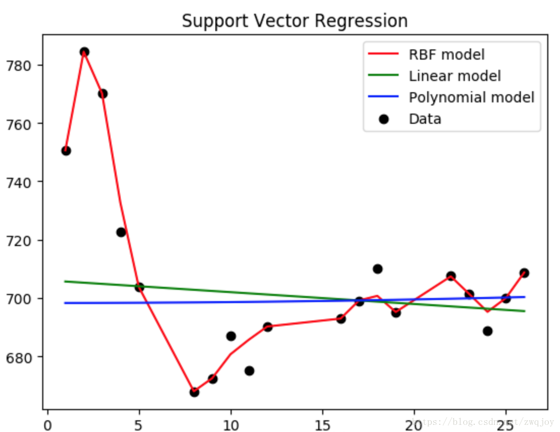
kernel:核函数的类型,一般常用的有’rbf’,’linear’,’poly’,等如图4-1-2-1所示,发现使用rbf参数时函数模型的拟合效果最好。
C:惩罚因子
C表征你有多么重视离群点,C越大越重视,越不想丢掉它们。C值大时对误差分类的惩罚增大,C值小时对误差分类的惩罚减小。当C越大,趋近无穷的时候,表示不允许分类误差的存在,margin越小,容易过拟合;当C趋于0时,表示我们不再关注分类是否正确,只要求margin越大,容易欠拟合。如图所示发现当使用1e3时最为适宜。
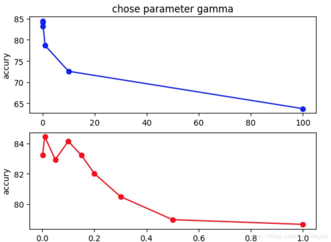
gamma:
是’rbf’,’poly’和’sigmoid’的核系数且gamma的值必须大于0。随着gamma的增大,存在对于测试集分类效果差而对训练分类效果好的情况,并且容易泛化误差出现过拟合。如图发现gamma=0.01时准确度最高。
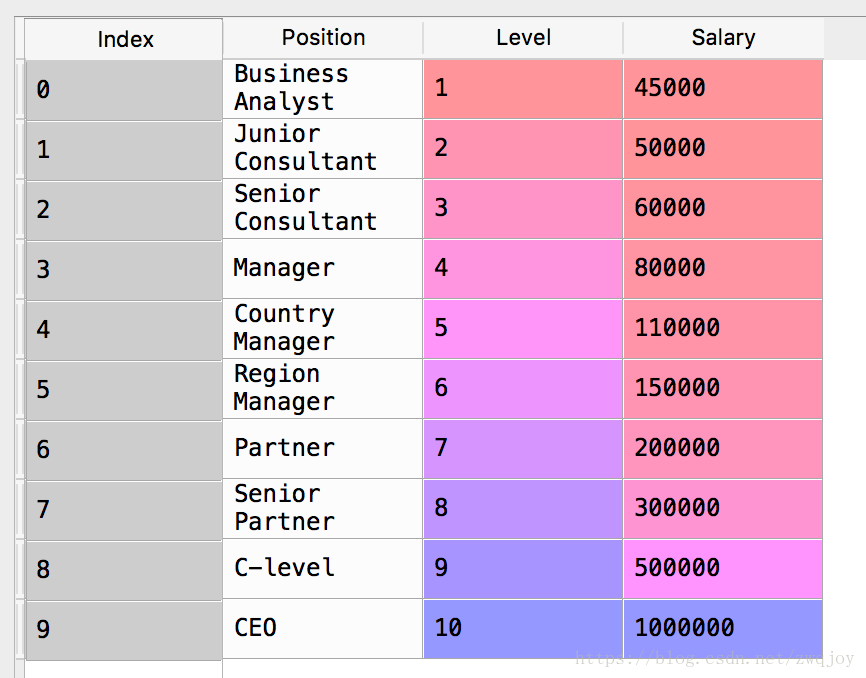
我们这次用的数据是公司内部不同的promotion level所对应的薪资
下面我们来看一下在Python中是如何实现的
import numpy as np
import matplotlib.pyplot as plt
import pandas as pd

dataset = pd.read_csv('Position_Salaries.csv')
X = dataset.iloc[:, 1:2].values
# 这里注意:1:2其实只有第一列,与1 的区别是这表示的是一个matrix矩阵,而非单一向量。
y = dataset.iloc[:, 2].values
接下来,处理数据:
# Reshape your data either using array.reshape(-1, 1) if your data has a single feature
# array.reshape(1, -1) if it contains a single sample.
X = np.reshape(X, (-1, 1))
y = np.reshape(y, (-1, 1))

# Feature Scaling
from sklearn.preprocessing import StandardScaler
sc_X = StandardScaler()
sc_y = StandardScaler()
X = sc_X.fit_transform(X)
y = sc_y.fit_transform(y)
接下来,进入正题,开始SVR回归:
# Fitting SVR to the dataset
from sklearn.svm import SVR
regressor = SVR(kernel = 'rbf')
regressor.fit(X, y)

# Predicting a new result
y_pred = regressor.predict(sc_X.transform(np.array([[6.5]])))
# 转换回正常预测值
y_pred = sc_y.inverse_transform(y_pred)
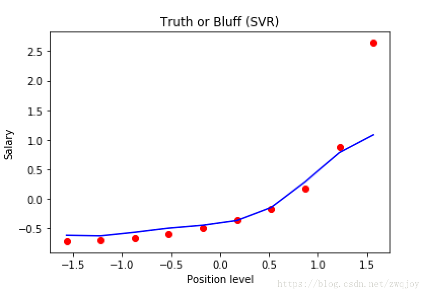
# 图像中显示
plt.scatter(X, y, color = 'red')
plt.plot(X, regressor.predict(X), color = 'blue')
plt.title('Truth or Bluff (SVR)')
plt.xlabel('Position level')
plt.ylabel('Salary')
plt.show()
# Visualising the SVR results (for higher resolution and smoother curve)
X_grid = np.arange(min(X), max(X), 0.01) # choice of 0.01 instead of 0.1 step because the data is feature scaled
X_grid = X_grid.reshape((len(X_grid), 1))
plt.scatter(X, y, color = 'red')
plt.plot(X_grid, regressor.predict(X_grid), color = 'blue')
plt.title('Truth or Bluff (SVR)')
plt.xlabel('Position level')
plt.ylabel('Salary')
plt.show()
