Sigmoid函数
首先介绍一下Sigmoid这个神奇的函数:
其图像如下:
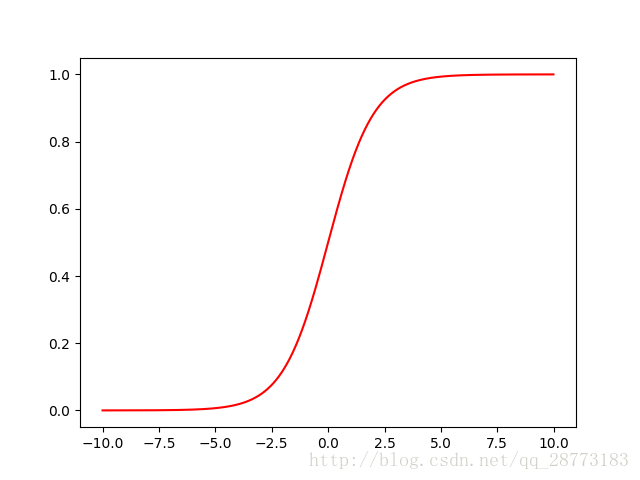
由图像可知,Sigmoid函数的值域在[0,1]之间,这对我们要做的分类是极其好的,因为我们完全可以从概率的角度来进行分类,单属于一个类的概率大于0.5时,我们就可以判定目标属于这个类。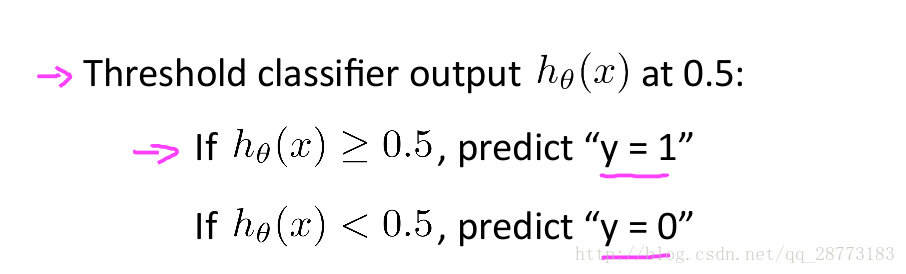
我们需要理解的是,Logistic Regression针对的是一个分类问题,而不是回归问题,之所以其名叫回归,主要是因为这个算法也是从线性回归中推出来的:
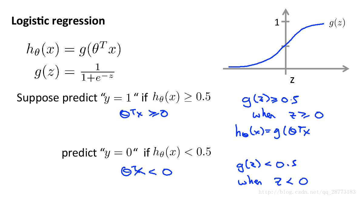
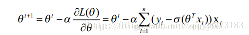
实际上只是换了我们线性回归的假设函数,其求解方法也是使用梯度下降算法(当然也可以用Conjugate Gradient、BFGS和L-BFGS算法,但这不是我们这次的重点)。
对于Logistic Regression算法,这里有个博客解释的很好:
Logistic Regression
我们的主要迭代步骤如下(求偏导的方法可以用参数替换来求):
Python实现
首先把效果图放出来(只迭代了100次,迭代次数多了,生成的GIF图太大了。。。):
代码如下:
# encoding:utf-8
###################
# Logistic Regression
# Author : FC
# Date : 2018/1/3
###################

from matplotlib import pyplot as plt
from matplotlib import animation
from numpy import *


#  读取.txt文件
def loadDataSet():
    dataMat = []
    labelMat = []
    fr = open('DataSet.txt')
    for line in fr.readlines():
        lineArr = line.strip().split()  # strip()函数删除空格,split()函数分割字符串存入到lineArr列表中
        dataMat.append([1.0, float(lineArr[0]), float(lineArr[1])])  # 这里的1.0是因为x0默认取1,整个运算过程是采用向量化计算
        labelMat.append(int(lineArr[2]))
    return dataMat, labelMat

# sigmoid函数
def sigmoid(inX):
    return 1/(1+exp(-inX))

# 梯度下降
def gradAscent(dataMatIn, classLabels, weights):
    # 向量化计算
    dataMatrix = mat(dataMatIn)
    classMatrix = mat(classLabels).transpose()
    weightsMatrix = mat(weights)
    h = sigmoid(dataMatrix*weightsMatrix)
    weightsMatrix = weightsMatrix-alpha*dataMatrix.transpose()*(h-classMatrix)
    return weightsMatrix
# 代价函数,用作收敛的判断
def costFunc(dataIn, labelIn, weights):
    errorCal = 0
    dataMatrix = mat(dataIn)
    weightsMatrix = mat(weights)
    h = sigmoid(dataMatrix * weightsMatrix)
    for i in range(m):
        errorCal += labelIn[i]*log(h[i])+(1-labelIn[i])*log(1-h[i])
    return errorCal

# 第一帧图像
def init():
    line.set_data([], [])
    x1=[]
    y1=[]
    x2 = []
    y2 = []
    for i in range(m):
        if datalabel[i] == 0:
            x1.append(float(data[i][1]))
            y1.append(float(data[i][2]))
        else:
            x2.append(float(data[i][1]))
            y2.append(float(data[i][2]))

    plt.plot(x1,y1,'ro')
    plt.plot(x2,y2,'g*')
    plt.grid(True)
    plt.xlabel('x')
    plt.ylabel('y')
    plt.title('Logistic Regression')
    return line, label

# 动作图像,横坐标是X1,z纵坐标是X2
def animate(i):
    x1 = -2
    x2 = 2
    y1 = -(float(Parm[i][0])-float(Parm[i][1])*x1)/float(Parm[i][2])
    y2 = -(float(Parm[i][0])-float(Parm[i][1])*x1)/float(Parm[i][2])
    line.set_data([x1, x2], [y1, y2])
    return line, label

# 初始化学习率,迭代阈值
alpha = 0.001
cnt = 0
esp = 0.001
error = 0
errorPre = 0
data, datalabel = loadDataSet()
m, n = shape(data)
theta = ones((n, 1))
Parm = []
Parm.append(theta)
for i in range(100):
    cnt += 1
    errorPre = costFunc(data, datalabel, theta)
    if abs(error - errorPre) < esp:
        break
    else:
        error = errorPre
    #  更新theta
    theta = gradAscent(data, datalabel, theta)
    Parm.append(theta)

# 画出动态图
fig,ax=plt.subplots()
line, = ax.plot([], [], 'g', lw=2)
label = ax.text([], [], '')

print(cnt)
init()
anim = animation.FuncAnimation(fig, animate, init_func=init, frames=cnt, interval=200, repeat=False, blit=True)

plt.show()
anim.save('LogisticRegression.gif', fps=4, writer='imagemagick')