Andrew Ng机器学习——线性回归(Linear Regression)和批处理梯度下降（BGD）

线性回归和梯度下降算法

关于线性回归和梯度下降算法，简单的说就是指这一类模型：输出是连续值，并且其假设函数是线性函数，所以其cost function很容易求偏导数。利用梯度下降的方法来求参数（局部最优解）。关于这一类算法的介绍推荐以下几个博客：
线性回归及梯度下降
BGD和SGD
本篇博客主要是分享一些可视化的python代码

python实现

首先是一个多特征的线性回归代码

# encoding:utf-8
# 作者：FC
# 日期：2017/12/25

# 数据集（Train DataSet）
x = [(1, 0, 3), (1, 1, 3), (1, 2, 3), (1, 3, 2), (1, 4, 4)]
y = [95.364, 97.217205, 75.195834, 60.105519, 49.342380]

# 设置迭代停止的条件
epsilon = 0.0001
max_itor = 10000

# 设置学习速率，迭代初始误差，迭代次数初始theta参数
alpha = 0.01
error_pre = 0
error = 0
cnt = 0
theta0 = 0; theta1 = 0;  theta2 = 0
m = len(x) # 数据集的长度
while True:
    cnt += 1
    error = 0
    # 计算代价函数
    for i in range(m):
        error += (theta0*x[i][0] + theta1*x[i][1] + theta2*x[i][2] - y[i])**2/(2*m)
    if abs(error - error_pre)<epsilon:
        break
    else:
        error_pre = error
    # 更新参数
    temp0=0;temp1=0;temp2=0
    for i in range(m):
        temp0 += (theta0*x[i][0]+theta1*x[i][1]+theta2*x[i][2]-y[i])*x[i][0]/m
        temp1 += (theta0 * x[i][0] + theta1 * x[i][1] + theta2 * x[i][2] - y[i]) * x[i][1] / m
        temp2 += (theta0 * x[i][0] + theta1 * x[i][1] + theta2 * x[i][2] - y[i]) * x[i][2] / m
    theta0 = theta0 - alpha*temp0
    theta1 = theta1 - alpha*temp1
    theta2 = theta2 - alpha*temp2

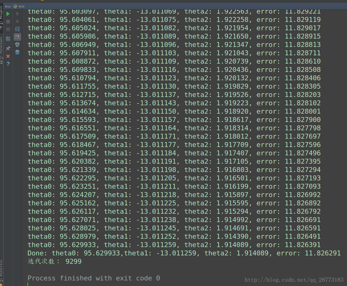
    print('theta0: %f, theta1: %f, theta2: %f, error: %f ' % (theta0,theta1,theta2,error))

print('Done: theta0: %f,theta1: %f, theta2: %f, error: %f'% (theta0,theta1,theta2,error))
print('迭代次数： %d' % cnt)

运行结果如下：

为了让整个过程更为形象，利用matplotlib库写了一个动态的一元线性回归实例，代码如下：

# -*-coding:utf-8
# Author:FC
# Date:2017/12/26
import numpy as np
from matplotlib import pyplot as plt
from matplotlib import animation
x = [1.5, 2.0, 2.5, 3.0, 3.5, 4.0, 6.0]
y = [64.5, 74.5, 84.5, 94.5, 114.5, 154.5, 184.5]
Parm = []


# 设置初始参数
eps = 0.0001  # 迭代阈值
alpha = 0.01  # 学习速率
theta0 = 0
theta1 = 0  # 初始theta
cnt = 0  # 迭代次数
error = 0
error_pre = 0
m = len(x)  # 训练集数量

def cost_func(a, b, theta0_new, theta1_new):
    J = 0  # 损失函数初始归零
    for i in range(len(a)):
        J += (theta0_new + theta1_new*a[i] - b[i])**2
    J = J/(2*len(a))
    return J

def Update_theta (a, b, theta0_new, theta1_new):
    k0 = 0
    k1 = 0
    theta0_update = 0
    theta1_update = 0
    for i in range(len(a)):
        k0 += (theta0_new + theta1_new*a[i] - b[i])
        k1 += (theta0_new + theta1_new*a[i] - b[i])*a[i]
    k0 = k0/len(a)
    k1 = k1//len(a)
    theta0_update = theta0_new - alpha*k0
    theta1_update = theta1_new - alpha*k1
    return theta0_update, theta1_update


while True:
    Parm.append([theta0,theta1])
    cnt += 1
    error = cost_func(x, y, theta0, theta1)
    if abs(error-error_pre) < eps:
        break
# 更新参数
    else:
        error_pre = error
        theta0, theta1 = Update_theta(x, y, theta0, theta1)


x_plot = np.arange(0.20, 0.1)
fig = plt.figure()
ax = plt.axes()
line, = ax.plot([], [], 'g', lw=2)
label = ax.text([], [], '')


def init():
    line.set_data([],[])
    plt.plot(x, y, 'ro')
    # plt.axis([-6, 6, -6, 6])
    plt.grid(True)
    plt.xlabel('x')
    plt.ylabel('y')
    plt.title('Linear Regression')
    return line, label

def animate(i):
    x1 = 0
    x2 = 18
    y1 = Parm[i][0]+x1*Parm[i][1]
    y2 = Parm[i][0] + x2 * Parm[i][1]
    line.set_data([x1, x2], [y1, y2])
    return line, label
anim = animation.FuncAnimation(fig, animate, init_func=init, frames= 100, interval=200, repeat=False, blit=True)

plt.show()
anim.save('Regression.gif', fps=4, writer='imagemagick')

结果如下：