参数:![]()
代价函数:![]()
代价函数偏导数:![]()
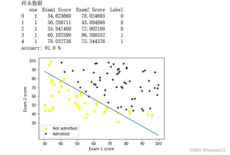
1 样本数据ex2data1.txt
本次算法的背景是,假如你是一个大学的管理者,你需要根据学生之前的成绩(两门科目)来预测该学生是否能进入该大学。
根据题意,我们不难分辨出这是一种二分类的逻辑回归,输入x有两种(科目1与科目2),输出有两种【能进入本大学(y=1)与不能进入本大学(y=0)】。输入测试样例以已经本文最前面贴出分别有两组数据。
具体样本数据如下:
34.62365962451697,78.0246928153624,0
30.28671076822607,43.89499752400101,0
35.84740876993872,72.90219802708364,0
60.18259938620976,86.30855209546826,1
79.0327360507101,75.3443764369103,1
45.08327747668339,56.3163717815305,0
61.10666453684766,96.51142588489624,1
75.02474556738889,46.55401354116538,1
76.09878670226257,87.42056971926803,1
84.43281996120035,43.53339331072109,1
95.86155507093572,38.22527805795094,0
75.01365838958247,30.60326323428011,0
82.30705337399482,76.48196330235604,1
69.36458875970939,97.71869196188608,1
39.53833914367223,76.03681085115882,0
53.9710521485623,89.20735013750205,1
69.07014406283025,52.74046973016765,1
67.94685547711617,46.67857410673128,0
70.66150955499435,92.92713789364831,1
76.97878372747498,47.57596364975532,1
67.37202754570876,42.83843832029179,0
89.67677575072079,65.79936592745237,1
50.534788289883,48.85581152764205,0
34.21206097786789,44.20952859866288,0
77.9240914545704,68.9723599933059,1
62.27101367004632,69.95445795447587,1
80.1901807509566,44.82162893218353,1
93.114388797442,38.80067033713209,0
61.83020602312595,50.25610789244621,0
38.78580379679423,64.99568095539578,0
61.379289447425,72.80788731317097,1
85.40451939411645,57.05198397627122,1
52.10797973193984,63.12762376881715,0
52.04540476831827,69.43286012045222,1
40.23689373545111,71.16774802184875,0
54.63510555424817,52.21388588061123,0
33.91550010906887,98.86943574220611,0
64.17698887494485,80.90806058670817,1
74.78925295941542,41.57341522824434,0
34.1836400264419,75.2377203360134,0
83.90239366249155,56.30804621605327,1
51.54772026906181,46.85629026349976,0
94.44336776917852,65.56892160559052,1
82.36875375713919,40.61825515970618,0
51.04775177128865,45.82270145776001,0
62.22267576120188,52.06099194836679,0
77.19303492601364,70.45820000180959,1
97.77159928000232,86.7278223300282,1
62.07306379667647,96.76882412413983,1
91.56497449807442,88.69629254546599,1
79.94481794066932,74.16311935043758,1
99.2725269292572,60.99903099844988,1
90.54671411399852,43.39060180650027,1
34.52451385320009,60.39634245837173,0
50.2864961189907,49.80453881323059,0
49.58667721632031,59.80895099453265,0
97.64563396007767,68.86157272420604,1
32.57720016809309,95.59854761387875,0
74.24869136721598,69.82457122657193,1
71.79646205863379,78.45356224515052,1
75.3956114656803,85.75993667331619,1
35.28611281526193,47.02051394723416,0
56.25381749711624,39.26147251058019,0
30.05882244669796,49.59297386723685,0
44.66826172480893,66.45008614558913,0
66.56089447242954,41.09209807936973,0
40.45755098375164,97.53518548909936,1
49.07256321908844,51.88321182073966,0
80.27957401466998,92.11606081344084,1
66.74671856944039,60.99139402740988,1
32.72283304060323,43.30717306430063,0
64.0393204150601,78.03168802018232,1
72.34649422579923,96.22759296761404,1
60.45788573918959,73.09499809758037,1
58.84095621726802,75.85844831279042,1
99.82785779692128,72.36925193383885,1
47.26426910848174,88.47586499559782,1
50.45815980285988,75.80985952982456,1
60.45555629271532,42.50840943572217,0
82.22666157785568,42.71987853716458,0
88.9138964166533,69.80378889835472,1
94.83450672430196,45.69430680250754,1
67.31925746917527,66.58935317747915,1
57.23870631569862,59.51428198012956,1
80.36675600171273,90.96014789746954,1
68.46852178591112,85.59430710452014,1
42.0754545384731,78.84478600148043,0
75.47770200533905,90.42453899753964,1
78.63542434898018,96.64742716885644,1
52.34800398794107,60.76950525602592,0
94.09433112516793,77.15910509073893,1
90.44855097096364,87.50879176484702,1
55.48216114069585,35.57070347228866,0
74.49269241843041,84.84513684930135,1
89.84580670720979,45.35828361091658,1
83.48916274498238,48.38028579728175,1
42.2617008099817,87.10385094025457,1
99.31500880510394,68.77540947206617,1
55.34001756003703,64.9319380069486,1
74.77589300092767,89.52981289513276,1
2 Python代码实现线性逻辑回归
import pandas as pd
import numpy as np
import matplotlib.pyplot as plt
import math
from collections import OrderedDict#用于导入数据的函数
def inputData():
#从txt文件中导入数据,注意最好标明数据的类型
data = pd.read_csv('D:/dataAnalysis/MachineLearning/ex2data1.txt'
,names = ['Exam1 Score','Exam2 Score','Label']
,dtype={0:float,1:float,2:int})
#插入一列全为1的列
data.insert(0,"one",[1 for i in range(0,data.shape[0])])
print('样本数据')
print(data.head())
#分别取出X和y
X=data.iloc[:,0:3].values
y=data.iloc[:,3].values
y=y.reshape(y.shape[0],1)
return X,y#用于最开始进行数据可视化的函数
def showData(X,y):
#分开考虑真实值y是1和0的行,分别绘制散点,并注意使用不同的label和marker
for i in range(0,X.shape[0]):
if(y[i,0]==1):
plt.scatter(X[i,1],X[i,2],marker='+',c='black',label='Admitted')
elif(y[i,0]==0):
plt.scatter(X[i,1],X[i,2],marker='o',c='yellow',label='Not admitted')
#设置坐标轴和图例
plt.xticks(np.arange(30,110,10))
plt.yticks(np.arange(30,110,10))
plt.xlabel('Exam 1 score')
plt.ylabel('Exam 2 score')
#因为上面绘制的散点不做处理的话,会有很多重复标签
#因此这里导入一个集合类消除重复的标签
handles, labels = plt.gca().get_legend_handles_labels() #获得标签
by_label = OrderedDict(zip(labels, handles)) #通过集合来删除重复的标签
plt.legend(by_label.values(), by_label.keys()) #显示图例
plt.show()#定义sigmoid函数
def sigmoid(z):
return 1/(1+np.exp(-z))#计算代价值的函数
def showCostsJ(X,y,theta,m):
#根据吴恩达老师上课讲的公式进行书写
#注意式子中加了1e-6次方是为了扩大精度,防止出现除0的警告
costsJ = ((y*np.log(sigmoid(X@theta)+ 1e-6))+((1-y)*np.log(1-sigmoid(X@theta)+ 1e-6))).sum()/(-m)
return costsJ#用于进行梯度下降的函数
def gradientDescent(X,y,theta,m,alpha,iterations):
for i in range(0,iterations): #进行迭代
# 进行向量化的计算。
#注意下面第二行使用X.T@ys可以替代掉之前的同步更新方式,写起来更简洁
ys=sigmoid(X@theta)-y
theta=theta-alpha*(X.T@ys)/m#以下完全代码,可以代替上面两行的代码
# temp0=theta[0][0]-alpha*(ys*(X[:,0].reshape(X.shape[0],1))).sum() #注意这里一定要将X[:,1]reshape成向量
# temp1=theta[1][0]-alpha*(ys*(X[:,1].reshape(X.shape[0],1))).sum()
# temp2=theta[2][0]-alpha*(ys*(X[:,2].reshape(X.shape[0],1))).sum()
# theta[0][0]=temp0 #进行同步更新θ0和θ1和θ2
# theta[1][0]=temp1
# theta[2][0]=temp2
return theta#对决策边界进行可视化的函数
def evaluateLogisticRegression(X,y,theta):
#这里和上面进行数据可视化的函数步骤是一样的,就不重复阐述了
for i in range(0,X.shape[0]):
if(y[i,0]==1):
plt.scatter(X[i,1],X[i,2],marker='+',c='black',label='Admitted')
elif(y[i,0]==0):
plt.scatter(X[i,1],X[i,2],marker='o',c='yellow',label='Not admitted')
plt.xticks(np.arange(30,110,10))
plt.yticks(np.arange(30,110,10))
plt.xlabel('Exam 1 score')
plt.ylabel('Exam 2 score')
handles, labels = plt.gca().get_legend_handles_labels()
by_label = OrderedDict(zip(labels, handles))
plt.legend(by_label.values(), by_label.keys())
minX=np.min(X[:,1]) #取得x1中的最小值
maxX=np.max(X[:,1]) #取得x1中的最大值
xx=np.linspace(minX,maxX,100) #创建等间距的数100个
yy=(theta[0][0]+theta[1][0]*xx)/(-theta[2][0]) #绘制决策边界
plt.plot(xx,yy)
plt.show()#利用训练集数据判断准确率的函数
def judge(X,y,theta):
ys=sigmoid(X@theta) #根据假设函数计算预测值ys
yanswer=y-ys #使用真实值y-预测值ys
yanswer=np.abs(yanswer) #对yanswer取绝对值
print('accuary:',(yanswer<0.5).sum()/y.shape[0]*100,'%') #计算准确率并打印结果
X,y = inputData() #输入数据
theta=np.zeros((3,1)) #初始化theta数组
alpha=0.004 #设定alpha值
iterations=200000 #设定迭代次数
theta=gradientDescent(X,y,theta,X.shape[0],alpha,iterations) #进行梯度下降
judge(X,y,theta) #计算准确率
evaluateLogisticRegression(X,y,theta) #决策边界可视化
运行结果如下: