PINN解偏微分方程实例3之Allen-Cahn方程
1. Allen-Cahn方程
考虑偏微分方程如下:
u t − 0.0001 u x x + 5 u 3 − 5 u = 0 u ( 0 , x ) = x 2 c o s ( π x ) u ( t , − 1 ) = u ( t , 1 ) u x ( t , − 1 ) = u x ( t , 1 ) \begin{align} \begin{aligned} & u_t - 0.0001u_{xx} + 5u^3 -5u = 0 \\ & u(0,x) = x^2cos(\pi x) \\ & u(t,-1) = u(t,1) \\ & u_x(t,-1) = u_x(t,1) \end{aligned} \end{align} ut−0.0001uxx+5u3−5u=0u(0,x)=x2cos(πx)u(t,−1)=u(t,1)ux(t,−1)=ux(t,1)
其中 x ∈ [ − 1 , 1 ] , t ∈ [ 0 , 1 ] . x\in[-1,1],t\in[0,1]. x∈[−1,1],t∈[0,1].这是一个带有周期性边界条件,初始条件的偏微分方程。这个方程主要用 P I N N [ 1 ] PINN^{[1]} PINN[1]论文中正向问题的离散时间模型求解。
2. 损失函数如下定义
S S E = S S E n + S S E b \begin{align} \begin{aligned} SSE = SSE_n + SSE_b \\ \end{aligned} \end{align} SSE=SSEn+SSEb
其中
S S E n = ∑ j = 1 q + 1 ∑ i = 1 N n ∣ u j n ( x n , i ) − u n , i ∣ 2 S S E b = ∑ i = 1 q ∣ u n + c i ( − 1 ) − u n + c i ( 1 ) ∣ 2 + ∣ u n + 1 ( − 1 ) − u n + 1 ( 1 ) ∣ 2 + ∑ i = 1 q ∣ u x n + c i ( − 1 ) − u x n + c i ( 1 ) ∣ 2 + ∣ u x n + 1 ( − 1 ) − u x n + 1 ( 1 ) ∣ 2 \begin{align} \begin{aligned} SSE_n &= \sum_{j=1}^{q+1}\sum_{i=1}^{N_n}|u_j^{n}(x^{n,i})-u^{n,i}|^2 \\ SSE_b &= \sum_{i=1}^{q} |u^{n+c_i}(-1)-u^{n+c_i}(1)|^2+ |u^{n+1}(-1)-u^{n+1}(1)|^2 \\ &+\sum_{i=1}^{q} |u_x^{n+c_i}(-1)-u_x^{n+c_i}(1)|^2+ |u_x^{n+1}(-1)-u_x^{n+1}(1)|^2 \\ \end{aligned} \end{align} SSEnSSEb=j=1∑q+1i=1∑Nn∣ujn(xn,i)−un,i∣2=i=1∑q∣un+ci(−1)−un+ci(1)∣2+∣un+1(−1)−un+1(1)∣2+i=1∑q∣uxn+ci(−1)−uxn+ci(1)∣2+∣uxn+1(−1)−uxn+1(1)∣2
这里 S S E b SSE_b SSEb是周期性边界损失, S S E n SSE_n SSEn可以理解为PDE损失, { x n , i , u n , i } ∣ i = 1 N n \{x^{n,i},u^{n,i}\}|_{i=1}^{N_n} {
xn,i,un,i}∣i=1Nn为 t n t^n tn时刻相应的数据点和真解。 u j n ( x n , i ) u_j^{n}(x^{n,i}) ujn(xn,i)利用公式(4)、(5)计算得到。
u n + c i = u n − Δ t ∑ j = 1 q a i j N [ u n + c j ] , i = 1 , 2 , . . . , q u n + 1 = u n − Δ t ∑ j = 1 q b j N [ u n + c j ] . \begin{align} \begin{aligned} u^{n+c_i} &= u^n - \Delta t \sum_{j=1}^q a_{ij} \mathcal{N}[u^{n+c_j}], \quad i=1,2,...,q \\ u^{n+1} &= u^n - \Delta t \sum_{j=1}^q b_{j} \mathcal{N}[u^{n+c_j}]. \end{aligned} \end{align} un+ciun+1=un−Δtj=1∑qaijN[un+cj],i=1,2,...,q=un−Δtj=1∑qbjN[un+cj].
公式(4)中 N [ u n + c j ] \mathcal{N}[u^{n+c_j}] N[un+cj]表达式如公式(5)所示。
N [ u n + c j ] = − 0.0001 u x x n + c j + 5 ( u n + c j ) 3 − 5 u n + c j \begin{align} \begin{aligned} \mathcal{N}[u^{n+c_j}] = -0.0001u_{xx}^{n+c_j} + 5(u^{n+c_j})^3 - 5u^{n+c_j} \end{aligned} \end{align} N[un+cj]=−0.0001uxxn+cj+5(un+cj)3−5un+cj
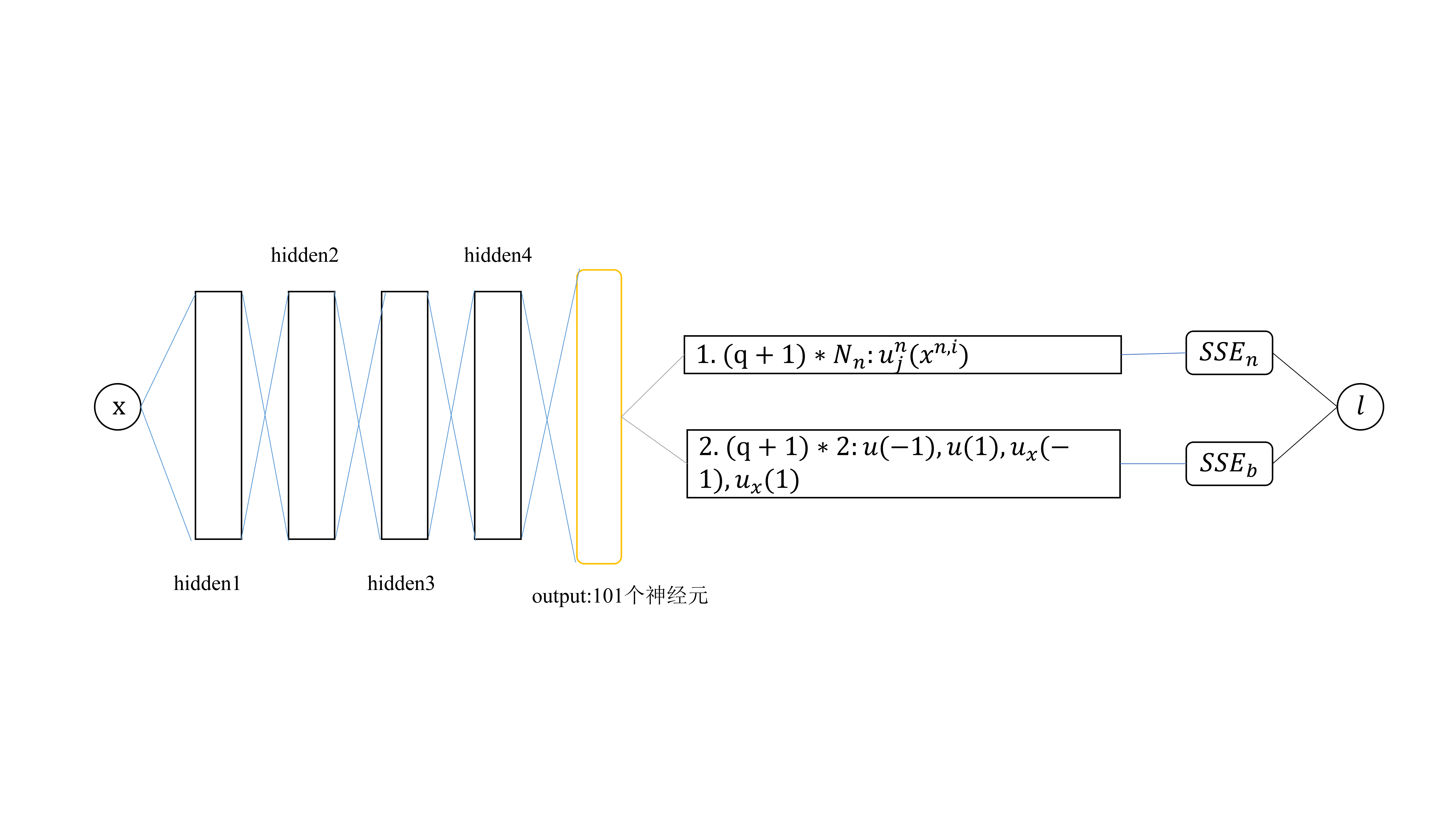
这里 N n = 200 , q = 100 , Δ t = 0.8 N_n=200,q=100,\Delta t=0.8 Nn=200,q=100,Δt=0.8。神经网络模型输入层包括一个神经元,四个100神经元的隐藏层,101个神经元的输出层。
3. 代码
代码参考下图进行理解。
代码参考https://github.com/maziarraissi/PINNs,原代码运行框架tensorflow1,这里将其改为tensorflow2上运行,代码如下:
"""
@author: Maziar Raissi
@Annotator:ST
计算t*x为[0,1]*[-1,1]区域上的真解,真解个数t*x为201*256
"""

import sys
sys.path.insert(0, '../../Utilities/')

import tensorflow.compat.v1 as tf   # tensorflow1.0代码迁移到2.0上运行,加上这两行
tf.disable_v2_behavior()

# import tensorflow as tf
import numpy as np
import matplotlib.pyplot as plt
import time
import scipy.io
from plotting import newfig, savefig
import matplotlib.gridspec as gridspec
from mpl_toolkits.axes_grid1 import make_axes_locatable

np.random.seed(1234)
tf.set_random_seed(1234)


class PhysicsInformedNN:
    # Initialize the class
    def __init__(self, x0, u0, x1, layers, dt, lb, ub, q):
        """
        input: 200个t=0.1时x坐标,x=-1,1 输入202个样本
        output: 每个坐标输出这个坐标在未来q个时间的解和t+dt时刻的解,输出维度分别为(200*101)(2*101)
        :param x0: 空间选定的200个点的x坐标值
        :param u0: 200个x在t=0.1时对应的u的精确解
        :param x1: 空间边界[[-1],[1]]
        :param layers: 神经网络各层神经元列表
        :param dt: 时间步长 0.8
        :param lb: -1
        :param ub: 1
        :param q: q阶龙格库达,即t方向取q个点的斜率的加权平均作为龙格库达法的平均斜率
        """
        self.lb = lb
        self.ub = ub

        self.x0 = x0
        self.x1 = x1

        self.u0 = u0

        self.layers = layers
        self.dt = dt
        self.q = max(q,1)

        # Initialize NN
        self.weights, self.biases = self.initialize_NN(layers)

        # Load IRK weights
        tmp = np.float32(np.loadtxt('../../Utilities/IRK_weights/Butcher_IRK%d.txt' % (q), ndmin = 2))
        self.IRK_weights = np.reshape(tmp[0:q**2+q], (q+1,q))
        self.IRK_times = tmp[q**2+q:]

        # tf placeholders and graph
        self.sess = tf.Session(config=tf.ConfigProto(allow_soft_placement=True,
                                                     log_device_placement=True))

        self.x0_tf = tf.placeholder(tf.float32, shape=(None, self.x0.shape[1]))
        self.x1_tf = tf.placeholder(tf.float32, shape=(None, self.x1.shape[1]))
        self.u0_tf = tf.placeholder(tf.float32, shape=(None, self.u0.shape[1]))
        self.dummy_x0_tf = tf.placeholder(tf.float32, shape=(None, self.q)) # dummy variable for fwd_gradients
        self.dummy_x1_tf = tf.placeholder(tf.float32, shape=(None, self.q+1)) # dummy variable for fwd_gradients

        self.U0_pred = self.net_U0(self.x0_tf) # N(200) x (q+1)  200个x内部点输入网络训练
        self.U1_pred, self.U1_x_pred= self.net_U1(self.x1_tf) # N1(=2) x (q+1)  x=-1,1 输入网络得到边界
        # self.U1_pred (2*101) 分别对应x=-1,1时的预测的dt内q个真解和一个u^{n+1}时的真解

        self.loss = tf.reduce_sum(tf.square(self.u0_tf - self.U0_pred)) + \
                    tf.reduce_sum(tf.square(self.U1_pred[0,:] - self.U1_pred[1,:])) + \
                    tf.reduce_sum(tf.square(self.U1_x_pred[0,:] - self.U1_x_pred[1,:]))

        # self.optimizer = tf.contrib.opt.ScipyOptimizerInterface(self.loss,
        #                                                         method = 'L-BFGS-B',
        #                                                         options = {'maxiter': 50000,
        #                                                                    'maxfun': 50000,
        #                                                                    'maxcor': 50,
        #                                                                    'maxls': 50,
        #                                                                    'ftol' : 1.0 * np.finfo(float).eps})

        self.optimizer_Adam = tf.train.AdamOptimizer()
        self.train_op_Adam = self.optimizer_Adam.minimize(self.loss)

        init = tf.global_variables_initializer()
        self.sess.run(init)

    def initialize_NN(self, layers):
        weights = []
        biases = []
        num_layers = len(layers)
        for l in range(0,num_layers-1):
            W = self.xavier_init(size=[layers[l], layers[l+1]])
            b = tf.Variable(tf.zeros([1,layers[l+1]], dtype=tf.float32), dtype=tf.float32)
            weights.append(W)
            biases.append(b)
        return weights, biases

    def xavier_init(self, size):
        in_dim = size[0]
        out_dim = size[1]
        xavier_stddev = np.sqrt(2/(in_dim + out_dim))
        return tf.Variable(tf.truncated_normal([in_dim, out_dim], stddev=xavier_stddev), dtype=tf.float32)

    def neural_net(self, X, weights, biases):
        num_layers = len(weights) + 1

        H = 2.0*(X - self.lb)/(self.ub - self.lb) - 1.0
        for l in range(0,num_layers-2):
            W = weights[l]
            b = biases[l]
            H = tf.tanh(tf.add(tf.matmul(H, W), b))
        W = weights[-1]
        b = biases[-1]
        Y = tf.add(tf.matmul(H, W), b)
        return Y

    def fwd_gradients_0(self, U, x):
        g = tf.gradients(U, x, grad_ys=self.dummy_x0_tf)[0]
        return tf.gradients(g, self.dummy_x0_tf)[0]

    def fwd_gradients_1(self, U, x):
        g = tf.gradients(U, x, grad_ys=self.dummy_x1_tf)[0]
        return tf.gradients(g, self.dummy_x1_tf)[0]

    def net_U0(self, x):
        U1 = self.neural_net(x, self.weights, self.biases)
        U = U1[:,:-1]
        U_x = self.fwd_gradients_0(U, x)
        U_xx = self.fwd_gradients_0(U_x, x)
        F = 5.0*U - 5.0*U**3 + 0.0001*U_xx
        U0 = U1 - self.dt*tf.matmul(F, self.IRK_weights.T)    # IRK_weights(101*100)  包括了Runde-Kutta方法参数a,b
        return U0

    def net_U1(self, x):
        U1 = self.neural_net(x, self.weights, self.biases)
        U1_x = self.fwd_gradients_1(U1, x)
        return U1, U1_x # N x (q+1)

    def callback(self, loss):
        print('Loss:', loss)

    def train(self, nIter):
        tf_dict = {

    self.x0_tf: self.x0, self.u0_tf: self.u0, self.x1_tf: self.x1,
                   self.dummy_x0_tf: np.ones((self.x0.shape[0], self.q)),
                   self.dummy_x1_tf: np.ones((self.x1.shape[0], self.q+1))}

        start_time = time.time()
        for it in range(nIter):
            self.sess.run(self.train_op_Adam, tf_dict)

            # Print
            if it % 10 == 0:
                elapsed = time.time() - start_time
                loss_value = self.sess.run(self.loss, tf_dict)
                print('It: %d, Loss: %.3e, Time: %.2f' %
                      (it, loss_value, elapsed))
                start_time = time.time()

        # self.optimizer.minimize(self.sess,
        #                         feed_dict = tf_dict,
        #                         fetches = [self.loss],
        #                         loss_callback = self.callback)

    def predict(self, x_star):

        U1_star = self.sess.run(self.U1_pred, {

    self.x1_tf: x_star})

        return U1_star


if __name__ == "__main__":

    q = 100
    layers = [1, 200, 200, 200, 200, q+1]
    lb = np.array([-1.0])
    ub = np.array([1.0])

    N = 200

    data = scipy.io.loadmat('../Data/AC.mat')

    t = data['tt'].flatten()[:,None]  # T(201) x 1  精确解时间坐标节点
    x = data['x'].flatten()[:,None]  # N(512) x 1  精确解空间坐标节点
    Exact = np.real(data['uu']).T  # T x N 精确解

    idx_t0 = 20
    idx_t1 = 180
    dt = t[idx_t1] - t[idx_t0]    # 时间步长0.8

    # Initial data
    noise_u0 = 0.0
    idx_x = np.random.choice(Exact.shape[1], N, replace=False)    # 随机选择空间200个点的下标索引
    x0 = x[idx_x,:]    # 空间200个点的x坐标值
    u0 = Exact[idx_t0:idx_t0+1,idx_x].T    # t=0.10时200个精确解
    u0 = u0 + noise_u0*np.std(u0)*np.random.randn(u0.shape[0], u0.shape[1])


    # Boudanry data
    x1 = np.vstack((lb,ub))

    # Test data
    x_star = x

    model = PhysicsInformedNN(x0, u0, x1, layers, dt, lb, ub, q)
    model.train(2)    # 10000

    U1_pred = model.predict(x_star)    # (512,101)

    error = np.linalg.norm(U1_pred[:,-1] - Exact[idx_t1,:], 2)/np.linalg.norm(Exact[idx_t1,:], 2)
    print('Error: %e' % (error))  # sqrt(sum_{i=1}^512 (u-u_{ext})) / sqrt(sum_{i=1}^512 (u_{ext}))  相对误差

    ######################################################################
    ############################# Plotting ###############################
    ######################################################################

    fig, ax = newfig(1.0, 1.2)
    ax.axis('off')

    ####### Row 0: h(t,x) ##################
    gs0 = gridspec.GridSpec(1, 2)
    gs0.update(top=1-0.06, bottom=1-1/2 + 0.1, left=0.15, right=0.85, wspace=0)
    ax = plt.subplot(gs0[:, :])

    h = ax.imshow(Exact.T, interpolation='nearest', cmap='seismic',
                  extent=[t.min(), t.max(), x_star.min(), x_star.max()],
                  origin='lower', aspect='auto')
    divider = make_axes_locatable(ax)
    cax = divider.append_axes("right", size="5%", pad=0.05)
    fig.colorbar(h, cax=cax)

    line = np.linspace(x.min(), x.max(), 2)[:,None]
    ax.plot(t[idx_t0]*np.ones((2,1)), line, 'w-', linewidth = 1)
    ax.plot(t[idx_t1]*np.ones((2,1)), line, 'w-', linewidth = 1)

    ax.set_xlabel('$t$')
    ax.set_ylabel('$x$')
    leg = ax.legend(frameon=False, loc = 'best')
    ax.set_title('$u(t,x)$', fontsize = 10)


    ####### Row 1: h(t,x) slices ##################
    gs1 = gridspec.GridSpec(1, 2)
    gs1.update(top=1-1/2-0.05, bottom=0.15, left=0.15, right=0.85, wspace=0.5)

    ax = plt.subplot(gs1[0, 0])
    ax.plot(x,Exact[idx_t0,:], 'b-', linewidth = 2)
    ax.plot(x0, u0, 'rx', linewidth = 2, label = 'Data')
    ax.set_xlabel('$x$')
    ax.set_ylabel('$u(t,x)$')
    ax.set_title('$t = %.2f$' % (t[idx_t0]), fontsize = 10)
    ax.set_xlim([lb-0.1, ub+0.1])
    ax.legend(loc='upper center', bbox_to_anchor=(0.8, -0.3), ncol=2, frameon=False)


    ax = plt.subplot(gs1[0, 1])
    ax.plot(x,Exact[idx_t1,:], 'b-', linewidth = 2, label = 'Exact')
    ax.plot(x_star, U1_pred[:,-1], 'r--', linewidth = 2, label = 'Prediction')
    ax.set_xlabel('$x$')
    ax.set_ylabel('$u(t,x)$')
    ax.set_title('$t = %.2f$' % (t[idx_t1]), fontsize = 10)
    ax.set_xlim([lb-0.1, ub+0.1])
    ax.legend(loc='upper center', bbox_to_anchor=(0.1, -0.3), ncol=2, frameon=False)

    savefig('./figures/retest/reAC')
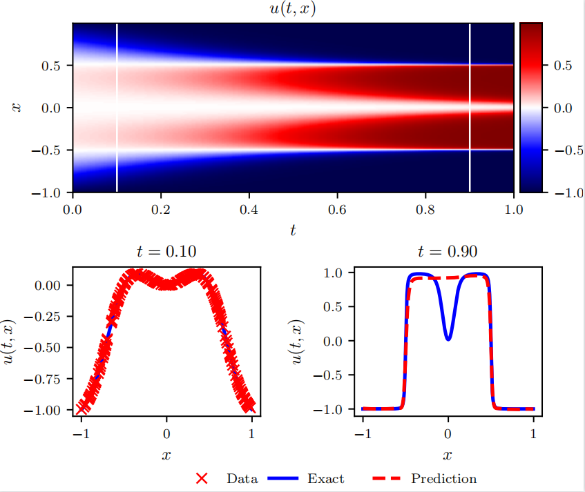
4. 实验细节及复现结果
这里使用4层全连接神经网络,输入层和输出层各两个神经元,输入层一个神经元代表 x x x坐标值,输出层101个神经元分别代表 [ u n + c 1 ( x ) , ⋯ , u n + c q ( x ) , u n + 1 ( x ) ] [u^{n+c_1}(x),\cdots,u^{n+c_q}(x),u^{n+1}(x)] [un+c1(x),⋯,un+cq(x),un+1(x)],隐藏层每层100个神经元。为了计算误差,作者提供了使用谱方法计算的 ( 256 ∗ 201 ) (256*201) (256∗201)个真解,其中第一维度代表空间 x x x,第二维度代表时间 t t t. 训练10000次之后输出结果如下:
It: 9970, Loss: 5.127e+00, Time: 0.08
It: 9980, Loss: 1.335e+01, Time: 0.07
It: 9990, Loss: 2.095e+01, Time: 0.07
Error: 2.470155e-01
这里误差是相对误差,计算公式如下:
E r r o r = ∣ ∣ U − U e x t ∣ ∣ 2 ∣ ∣ U e x t ∣ ∣ 2 \begin{align} \begin{aligned} Error = \frac{||U-U_{ext}||_2}{||U_{ext}||_2} \end{aligned} \end{align} Error=∣∣Uext∣∣2∣∣U−Uext∣∣2
其中 U ∈ R 512 × 1 , U e x t ∈ R 512 × 1 U \in \mathbb{R}^{512 \times 1},U_{ext}\in \mathbb{R}^{512 \times 1} U∈R512×1,Uext∈R512×1,前者为 t = 0.9 t=0.9 t=0.9时PINN预测的解,后者为 t = 0.9 t=0.9 t=0.9时计算的精确解。复现结果图如下:
论文中结果如下:
