改善深层神经网络第一周-Initialization

Initialization

Welcome to the first assignment of “Improving Deep Neural Networks”.

Training your neural network requires specifying an initial value of the weights. A well chosen initialization method will help learning. (训练你的神经网络需要指定权重的初始值。精心挑选的初始化方法将有助于学习。)

If you completed the previous course of this specialization, you probably followed our instructions for weight initialization, and it has worked out so far. But how do you choose the initialization for a new neural network? In this notebook, you will see how different initializations lead to different results. (如果你完成了这个专业化的前一个课程，你可能按照我们的指导进行体重初始化，到目前为止它已经成功。但是，你如何选择一个新的神经网络的初始化？在这个笔记本中，你会看到不同的初始化会带来不同的结果。)

A well chosen initialization can: 
- Speed up the convergence of gradient descent(加快梯度下降的趋势) 
- Increase the odds of gradient descent converging to a lower training (and generalization) error (增加梯度下降收敛到较低的训练（和泛化）错误的几率)

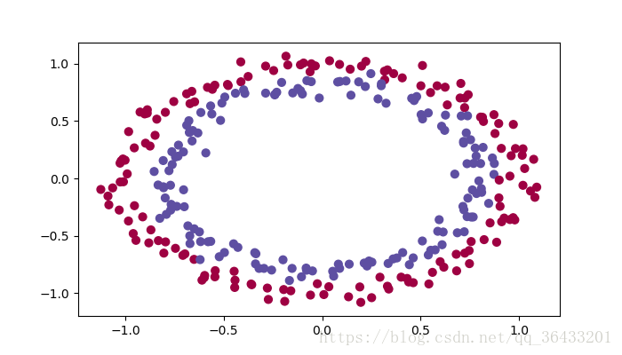
To get started, run the following cell to load the packages and the planar dataset you will try to classify.

import numpy as np
import matplotlib.pyplot as plt
import sklearn
import sklearn.datasets
from init_utils import sigmoid, relu, compute_loss, forward_propagation, backward_propagation
from init_utils import update_parameters, predict, load_dataset, plot_decision_boundary, predict_dec
#%matplotlib inline
plt.rcParams['figure.figsize'] = (7.0, 4.0) # set default size of plots
plt.rcParams['image.interpolation'] = 'nearest'
plt.rcParams['image.cmap'] = 'gray'

# load image dataset: blue/red dots in circles
train_X, train_Y, test_X, test_Y = load_dataset()
plt.show()

     

1 - Neural Network model

You will use a 3-layer neural network (already implemented for you). Here are the initialization methods you will experiment with: 
- Zeros initialization – setting initialization = "zeros" in the input argument. 
- Random initialization – setting initialization = "random" in the input argument. This initializes the weights to large random values. (这将权重初始化为大的随机值) 
- He initialization – setting initialization = "he" in the input argument. This initializes the weights to random values scaled according to a paper by He et al., 2015. (这将权重初始化为根据He等人，2015年的论文缩放的随机值)

Instructions: Please quickly read over the code below, and run it. In the next part you will implement the three initialization methods that this model() calls.

2 - Zero initialization

Exercise: Implement the following function to initialize all parameters to zeros. You’ll see later that this does not work well since it fails to “break symmetry”, but lets try it anyway and see what happens. Use np.zeros((..,..)) with the correct shapes.(实现以下功能将所有参数初始化为零。稍后你会看到，这不能很好地工作，因为它不能“破坏对称性”，而是让我们尝试一下，看看会发生什么。使用正确形状的np.zeros（（..，..））)

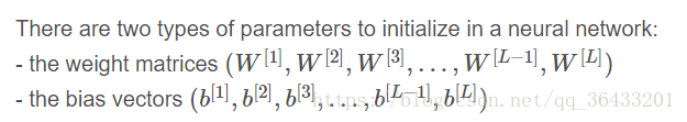
def initialize_parameters_zeros(layers_dims):
    """
    Arguments:
    layer_dims -- python array (list) containing the size of each layer.

    Returns:
    parameters -- python dictionary containing your parameters "W1", "b1", ..., "WL", "bL":
                    W1 -- weight matrix of shape (layers_dims[1], layers_dims[0])
                    b1 -- bias vector of shape (layers_dims[1], 1)
                    ...
                    WL -- weight matrix of shape (layers_dims[L], layers_dims[L-1])
                    bL -- bias vector of shape (layers_dims[L], 1)
    """

    parameters = {}
    L = len(layers_dims)            # number of layers in the network

    for l in range(1, L):
        ### START CODE HERE ### (≈ 2 lines of code)
        parameters['W' + str(l)] = np.zeros((layers_dims[l],layers_dims[l-1]))
        parameters['b' + str(l)] = np.zeros((layers_dims[l],1))
        ### END CODE HERE ###
    return parameters
if __name__ == '__main__':
    model(train_X,train_Y,initialization='zeros')

  parameters = initialize_parameters_zeros([3, 2, 1])
  print("W1 = " + str(parameters["W1"]))
  print("b1 = " + str(parameters["b1"]))
  print("W2 = " + str(parameters["W2"]))
  print("b2 = " + str(parameters["b2"]))

结果：

W1 = [[0. 0. 0.]
      [0. 0. 0.]]
b1 = [[0.]
      [0.]]
W2 = [[0. 0.]]
b2 = [[0.]]

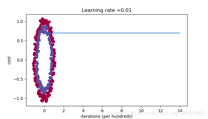
Run the following code to train your model on 15,000 iterations using zeros initialization.

parameters = model(train_X, train_Y, initialization="zeros")
print("On the train set:")
predictions_train = predict(train_X, train_Y, parameters)
print("On the test set:")
predictions_test = predict(test_X, test_Y, parameters)

结果：

Cost after iteration 0: 0.6931471805599453
Cost after iteration 1000: 0.6931471805599453
Cost after iteration 2000: 0.6931471805599453
Cost after iteration 3000: 0.6931471805599453
Cost after iteration 4000: 0.6931471805599453
Cost after iteration 5000: 0.6931471805599453
Cost after iteration 6000: 0.6931471805599453
Cost after iteration 7000: 0.6931471805599453
Cost after iteration 8000: 0.6931471805599453
Cost after iteration 9000: 0.6931471805599453
Cost after iteration 10000: 0.6931471805599455
Cost after iteration 11000: 0.6931471805599453
Cost after iteration 12000: 0.6931471805599453
Cost after iteration 13000: 0.6931471805599453
Cost after iteration 14000: 0.6931471805599453
On the train set:
Accuracy: 0.5
On the test set:

Accuracy: 0.5

The performance is really bad, and the cost does not really decrease, and the algorithm performs no better than random guessing. Why? Lets look at the details of the predictions and the decision boundary(性能非常糟糕，成本并没有真正降低，算法也没有比随机猜测更好。为什么？让我们看看预测和决策边界的细节):

print("predictions_train = " + str(predictions_train))
print("predictions_test = " + str(predictions_test))

结果：

predictions_train = [[0 0 0 0 0 0 0 0 0 0 0 0 0 0 0 0 0 0 0 0 0 0 0 0 0 0 0 0 0 0 0 0 0 0 0 0
                      0 0 0 0 0 0 0 0 0 0 0 0 0 0 0 0 0 0 0 0 0 0 0 0 0 0 0 0 0 0 0 0 0 0 0 0
                      0 0 0 0 0 0 0 0 0 0 0 0 0 0 0 0 0 0 0 0 0 0 0 0 0 0 0 0 0 0 0 0 0 0 0 0
                      0 0 0 0 0 0 0 0 0 0 0 0 0 0 0 0 0 0 0 0 0 0 0 0 0 0 0 0 0 0 0 0 0 0 0 0
                      0 0 0 0 0 0 0 0 0 0 0 0 0 0 0 0 0 0 0 0 0 0 0 0 0 0 0 0 0 0 0 0 0 0 0 0
                      0 0 0 0 0 0 0 0 0 0 0 0 0 0 0 0 0 0 0 0 0 0 0 0 0 0 0 0 0 0 0 0 0 0 0 0
                      0 0 0 0 0 0 0 0 0 0 0 0 0 0 0 0 0 0 0 0 0 0 0 0 0 0 0 0 0 0 0 0 0 0 0 0
                      0 0 0 0 0 0 0 0 0 0 0 0 0 0 0 0 0 0 0 0 0 0 0 0 0 0 0 0 0 0 0 0 0 0 0 0
                      0 0 0 0 0 0 0 0 0 0 0 0]]
predictions_test = [[0 0 0 0 0 0 0 0 0 0 0 0 0 0 0 0 0 0 0 0 0 0 0 0 0 0 0 0 0 0 0 0 0 0 0 0
                     0 0 0 0 0 0 0 0 0 0 0 0 0 0 0 0 0 0 0 0 0 0 0 0 0 0 0 0 0 0 0 0 0 0 0 0
                     0 0 0 0 0 0 0 0 0 0 0 0 0 0 0 0 0 0 0 0 0 0 0 0 0 0 0 0]]

axes = plt.gca()
axes.set_xlim([-1.5, 1.5])
axes.set_ylim([-1.5, 1.5])
plot_decision_boundary(lambda x: predict_dec(parameters, x.T), train_X, np.squeeze(train_Y))

                                

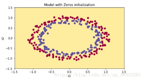
The model is predicting 0 for every example.

In general, initializing all the weights to zero results in the network failing to break symmetry. This means that every neuron in each layer will learn the same thing, and you might as well be training a neural network with $n^{\left[l\right]}=1$ for every layer, and the network is no more powerful than a linear classifier such as logistic regression. (一般来说，将所有权重初始化为零将导致网络无法破坏对称性。这意味着每一层中的每一个神经元都会学到相同的东西，而且你也可以用每一层的$n^{\left[l\right]}=1$来训练一个神经网络，并且网络没有线性强大分类器如逻辑回归)

What you should remember : 
- The weights  $W^{\left[l\right]}$  should be initialized randomly to break symmetry. ( 应该随机地初始化权重$W^{\left[l\right]}$以破坏对称性 ) 
- It is however okay to initialize the biases  $b^{\left[l\right]}$  to zeros. Symmetry is still broken so long as  $W^{\left[l\right]}$  is initialized randomly. ( 然而，将偏置$b^{\left[l\right]}$初始化为零是可以的。只要$W^{\left[l\right]}$

被随机初始化，对称性仍然被打破)

3 - Random initialization

To break symmetry, lets intialize the weights randomly. Following random initialization, each neuron can then proceed to learn a different function of its inputs. In this exercise, you will see what happens if the weights are intialized randomly, but to very large values. (为了打破对称，让随机初始化权重。随机初始化之后，每个神经元可以继续学习其输入的不同功能。在这个练习中，你会看到如果权重是随机初始化会发生什么，但是会发生什么)

Exercise: Implement the following function to initialize your weights to large random values (scaled by *10) and your biases to zeros. Use np.random.randn(..,..) * 10 for weights and np.zeros((.., ..)) for biases. We are using a fixed np.random.seed(..) to make sure your “random” weights match ours, so don’t worry if running several times your code gives you always the same initial values for the parameters. (实现以下功能，将您的权重初始化为较大的随机值（由*10缩放），并将偏差初始化为零。使用np.random.randn（..，..）* 10作为权重和np.zeros（（..，..））偏差。我们正在使用一个固定的np.random.seed（..）来确保你的“随机”权重符合我们的要求，所以不用担心，如果运行几次你的代码给你的参数总是相同的初始值。)

def initialize_parameters_random(layers_dims):
    """
    Arguments:
    layer_dims -- python array (list) containing the size of each layer.

    Returns:
    parameters -- python dictionary containing your parameters "W1", "b1", ..., "WL", "bL":
                    W1 -- weight matrix of shape (layers_dims[1], layers_dims[0])
                    b1 -- bias vector of shape (layers_dims[1], 1)
                    ...
                    WL -- weight matrix of shape (layers_dims[L], layers_dims[L-1])
                    bL -- bias vector of shape (layers_dims[L], 1)
    """

    np.random.seed(3)               # This seed makes sure your "random" numbers will be the as ours
    parameters = {}
    L = len(layers_dims)            # integer representing the number of layers

    for l in range(1, L):
        ### START CODE HERE ### (≈ 2 lines of code)
        parameters['W' + str(l)] = np.random.randn(layers_dims[l],layers_dims[l-1])*10
        parameters['b' + str(l)] = np.zeros((layers_dims[l],1))
        ### END CODE HERE ###

    return parameters
if __name__ == '__main__':
    parameters = initialize_parameters_random([3, 2, 1])
    print("W1 = " + str(parameters["W1"]))
    print("b1 = " + str(parameters["b1"]))
    print("W2 = " + str(parameters["W2"]))
    print("b2 = " + str(parameters["b2"]))

运行结果：

W1 = [[17.88628473   4.36509851   0.96497468]
      [-18.63492703 - 2.77388203 - 3.54758979]]
b1 = [[0.]
      [0.]]
W2 = [[-0.82741481 - 6.27000677]]
b2 = [[0.]]

Run the following code to train your model on 15,000 iterations using random initialization.

parameters = model(train_X, train_Y, initialization="random")
print("On the train set:")
predictions_train = predict(train_X, train_Y, parameters)
print("On the test set:")
predictions_test = predict(test_X, test_Y, parameters)

运行结果：

Cost after iteration 0: inf
Cost after iteration 1000: 0.6247924745506072
Cost after iteration 2000: 0.5980258056061102
Cost after iteration 3000: 0.5637539062842213
Cost after iteration 4000: 0.5501256393526495
Cost after iteration 5000: 0.5443826306793814
Cost after iteration 6000: 0.5373895855049121
Cost after iteration 7000: 0.47157999220550006
Cost after iteration 8000: 0.39770475516243037
Cost after iteration 9000: 0.3934560146692851
Cost after iteration 10000: 0.3920227137490125
Cost after iteration 11000: 0.38913700035966736
Cost after iteration 12000: 0.3861358766546214
Cost after iteration 13000: 0.38497629552893475
Cost after iteration 14000: 0.38276694641706693

.      

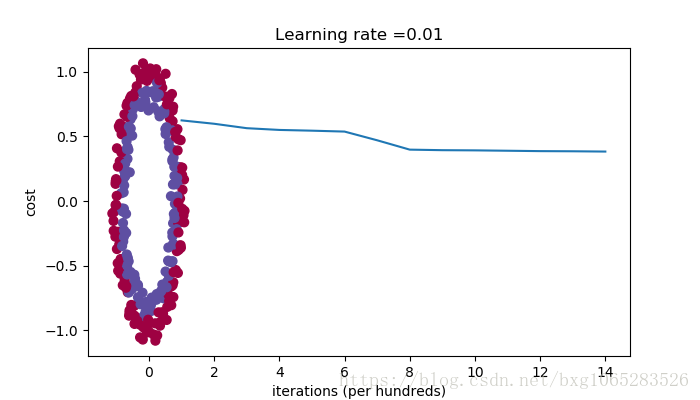
On the train set:
Accuracy: 0.83
On the test set:
Accuracy: 0.86

If you see “inf” as the cost after the iteration 0, this is because of numerical roundoff; a more numerically sophisticated implementation would fix this. But this isn’t worth worrying about for our purposes. (如果您看到“inf”作为迭代0之后的成本，这是因为数值舍入;一个更复杂的实现可以解决这个问题。但是这不值得为我们的目的而担心。)

Anyway, it looks like you have broken symmetry, and this gives better results. than before. The model is no longer outputting all 0s. (无论如何，看起来你已经破坏了对称性，而这样做会有更好的结果。比以前。该模型不再输出全0。)

[[1 0 1 1 0 0 1 1 1 1 1 0 1 0 0 1 0 1 1 0 0 0 1 0 1 1 1 1 1 1 0 1 1 0 0 1
  1 1 1 1 1 1 1 0 1 1 1 1 0 1 0 1 1 1 1 0 0 1 1 1 1 0 1 1 0 1 0 1 1 1 1 0
  0 0 0 0 1 0 1 0 1 1 1 0 0 1 1 1 1 1 1 0 0 1 1 1 0 1 1 0 1 0 1 1 0 1 1 0
  1 0 1 1 0 0 1 0 0 1 1 0 1 1 1 0 1 0 0 1 0 1 1 1 1 1 1 1 0 1 1 0 0 1 1 0
  0 0 1 0 1 0 1 0 1 1 1 0 0 1 1 1 1 0 1 1 0 1 0 1 1 0 1 0 1 1 1 1 0 1 1 1
  1 0 1 0 1 0 1 1 1 1 0 1 1 0 1 1 0 1 1 0 1 0 1 1 1 0 1 1 1 0 1 0 1 0 0 1
  0 1 1 0 1 1 0 1 1 0 1 1 1 0 1 1 1 1 0 1 0 0 1 1 0 1 1 1 0 0 0 1 1 0 1 1
  1 1 0 1 1 0 1 1 1 0 0 1 0 0 0 1 0 0 0 1 1 1 1 0 0 0 0 1 1 1 1 0 0 1 1 1
  1 1 1 1 0 0 0 1 1 1 1 0]]
[[1 1 1 1 0 1 0 1 1 0 1 1 1 0 0 0 0 1 0 1 0 0 1 0 1 0 1 1 1 1 1 0 0 0 0 1
  0 1 1 0 0 1 1 1 1 1 0 1 1 1 0 1 0 1 1 0 1 0 1 0 1 1 1 1 1 1 1 1 1 0 1 0
  1 1 1 1 1 0 1 0 0 1 0 0 0 1 1 0 1 1 0 0 0 1 1 0 1 1 0 0]]

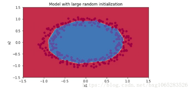
plt.title("Model with large random initialization")
axes = plt.gca()
axes.set_xlim([-1.5, 1.5])
axes.set_ylim([-1.5, 1.5])
plot_decision_boundary(lambda x: predict_dec(parameters, x.T), train_X, np.squeeze(train_Y))

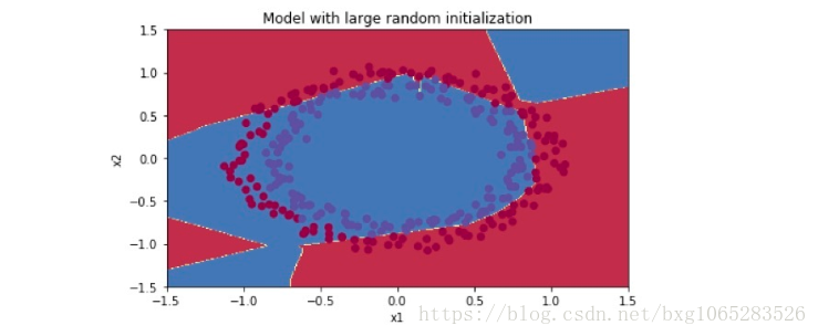
Observations: 

- The cost starts very high. This is because with large random-valued weights, the last activation (sigmoid) outputs results that are very close to 0 or 1 for some examples, and when it gets that example wrong it incurs a very high loss for that example. Indeed, when  $\log \left(a^{\left[3\right]}\right)=\log \left(0\right)$, the loss goes to infinity.( 成本开始非常高。这是因为对于大的随机值权重，最后一次激活（sigmoid）输出的结果非常接近于0或1，并且在得到这个例子的错误时，这个例子会导致非常高的损失。事实上，当$\log \left(a^{\left[3\right]}\right)=\log \left(0\right)$时，损失会变成无穷大) 
- Poor initialization can lead to vanishing/exploding gradients, which also slows down the optimization algorithm.( 初始化不良会导致渐变/爆炸渐变，这也会减慢优化算法的速度) 

- If you train this network longer you will see better results, but initializing with overly large random numbers slows down the optimization.(如果你长时间训练这个网络，你会看到更好的结果，但是用过大的随机数初始化会减慢优化速度)

4 - He initialization

In summary : 
- Initializing weights to very large random values does not work well. ( 将权重初始化为非常大的随机值效果不佳 ) 
- Hopefully intializing with small random values does better. The important question is: how small should be these random values be? Lets find out in the next part! ( 希望用小的随机值进行初始化会更好。重要的问题是这些随机值应该小到多少？让我们来看看下一部分！ )

Finally, try “He Initialization”; this is named for the first author of He et al., 2015. (If you have heard of “Xavier initialization”, this is similar except Xavier initialization uses a scaling factor for the weights $W^{\left[l\right]}$ of sqrt(1./layers_dims[l-1]) where He initialization would use sqrt(2./layers_dims[l-1]).)(最后，尝试“”He Initialization””; （如果您已经听说过“Xavier初始化”，那么除了Xavier初始化使用一个比例因子来计算“Xavier”的权重$W^{\left[l\right]}$以外，sqrt(1./layers_dims[l-1])在”He Initialization”将使用sqrt（2./layers_dims [l-1]）。）)

Exercise: Implement the following function to initialize your parameters with He initialization.

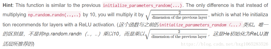
def initialize_parameters_he(layers_dims):
    """
    Arguments:
    layer_dims -- python array (list) containing the size of each layer.

    Returns:
    parameters -- python dictionary containing your parameters "W1", "b1", ..., "WL", "bL":
                    W1 -- weight matrix of shape (layers_dims[1], layers_dims[0])
                    b1 -- bias vector of shape (layers_dims[1], 1)
                    ...
                    WL -- weight matrix of shape (layers_dims[L], layers_dims[L-1])
                    bL -- bias vector of shape (layers_dims[L], 1)
    """

    np.random.seed(3)
    parameters = {}
    L = len(layers_dims) - 1 # integer representing the number of layers

    for l in range(1, L + 1):
        ### START CODE HERE ### (≈ 2 lines of code)
        parameters['W' + str(l)] = np.random.randn(layers_dims[l],layers_dims[l-1]) * np.sqrt(2./layers_dims[l-1])
        parameters['b' + str(l)] = np.zeros((layers_dims[l],1))
        ### END CODE HERE ###

    return parameters
if __name__ == '__main__':
    parameters = initialize_parameters_he([2, 4, 1])
    print("W1 = " + str(parameters["W1"]))
    print("b1 = " + str(parameters["b1"]))
    print("W2 = " + str(parameters["W2"]))
    print("b2 = " + str(parameters["b2"]))

W1 = [[1.78862847  0.43650985]
      [0.09649747 - 1.8634927]
      [-0.2773882 - 0.35475898]
      [-0.08274148 - 0.62700068]]
b1 = [[0.]
      [0.]
      [0.]
      [0.]]
W2 = [[-0.03098412 - 0.33744411 - 0.92904268  0.62552248]]
b2 = [[0.]]

Run the following code to train your model on 15,000 iterations using He initialization.

parameters = model(train_X, train_Y, initialization="he")
print("On the train set:")
predictions_train = predict(train_X, train_Y, parameters)
print("On the test set:")
predictions_test = predict(test_X, test_Y, parameters)

Cost after iteration 0: 0.8830537463419761
Cost after iteration 1000: 0.6879825919728063
Cost after iteration 2000: 0.6751286264523371
Cost after iteration 3000: 0.6526117768893805
Cost after iteration 4000: 0.6082958970572938
Cost after iteration 5000: 0.5304944491717495
Cost after iteration 6000: 0.4138645817071794
Cost after iteration 7000: 0.3117803464844441
Cost after iteration 8000: 0.23696215330322562
Cost after iteration 9000: 0.1859728720920684
Cost after iteration 10000: 0.15015556280371808
Cost after iteration 11000: 0.12325079292273551
Cost after iteration 12000: 0.09917746546525937
Cost after iteration 13000: 0.08457055954024283
Cost after iteration 14000: 0.07357895962677366

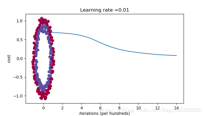
On the train set:
Accuracy: 0.9933333333333333
On the test set:
Accuracy: 0.96

plt.title("Model with He initialization")
axes = plt.gca()
axes.set_xlim([-1.5, 1.5])
axes.set_ylim([-1.5, 1.5])
plot_decision_boundary(lambda x: predict_dec(parameters, x.T), train_X, np.squeeze(train_Y))

                            

Observations: 
- The model with He initialization separates the blue and the red dots very well in a small number of iterations.

5 - Conclusions

You have seen three different types of initializations. For the same number of iterations and same hyperparameters the comparison is:

**Model**	**Train accuracy**	**Problem/Comment**
3-layer NN with zeros initialization	50%	fails to break symmetry
3-layer NN with large random initialization	83%	too large weights
3-layer NN with He initialization	99%	recommended method

What you should remember from this notebook: 
- Different initializations lead to different results(不同的初始化导致不同的结果) 
- Random initialization is used to break symmetry and make sure different hidden units can learn different things(随机初始化用于破坏对称性，并确保不同的隐藏单元可以学习不同的东西) 
- Don’t intialize to values that are too large(不要初始化太大的值) 
- He initialization works well for networks with ReLU activations. (他初始化适用于ReLU激活的网络)